9.34 A Black-Scholes for Beliefs: Logit Jump-Diffusion and Tradable Belief-Vol
Prediction markets have no Black-Scholes. A recent paper builds one: model log-odds as a jump-diffusion, force the price to be a martingale, trade what's left. Clean theory, thin evidence.
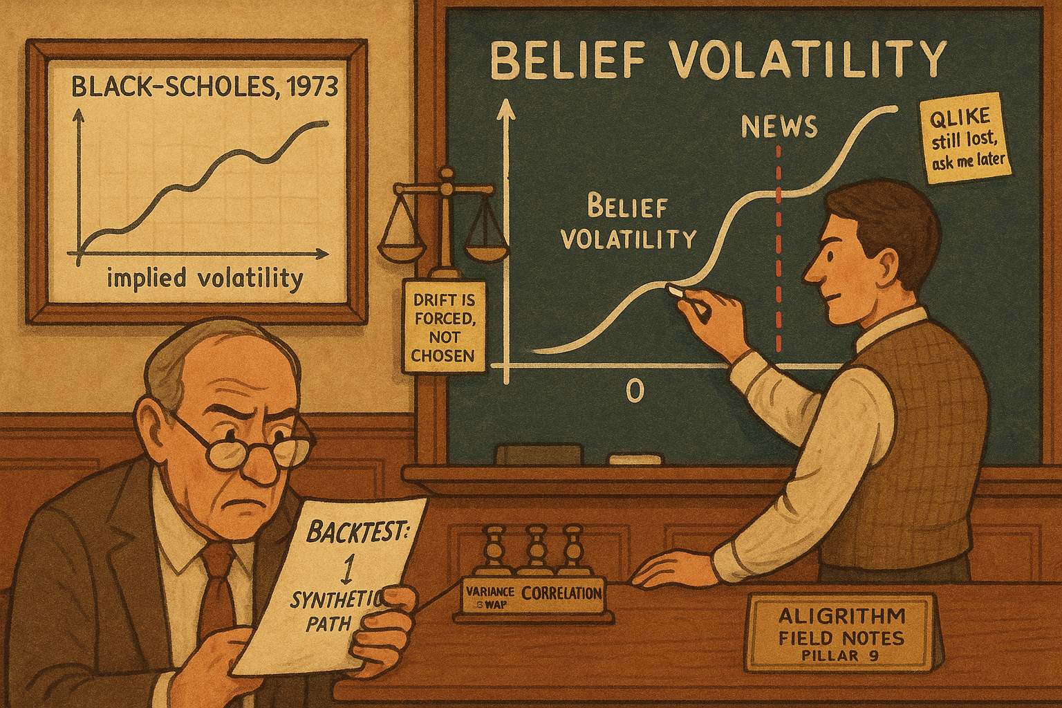
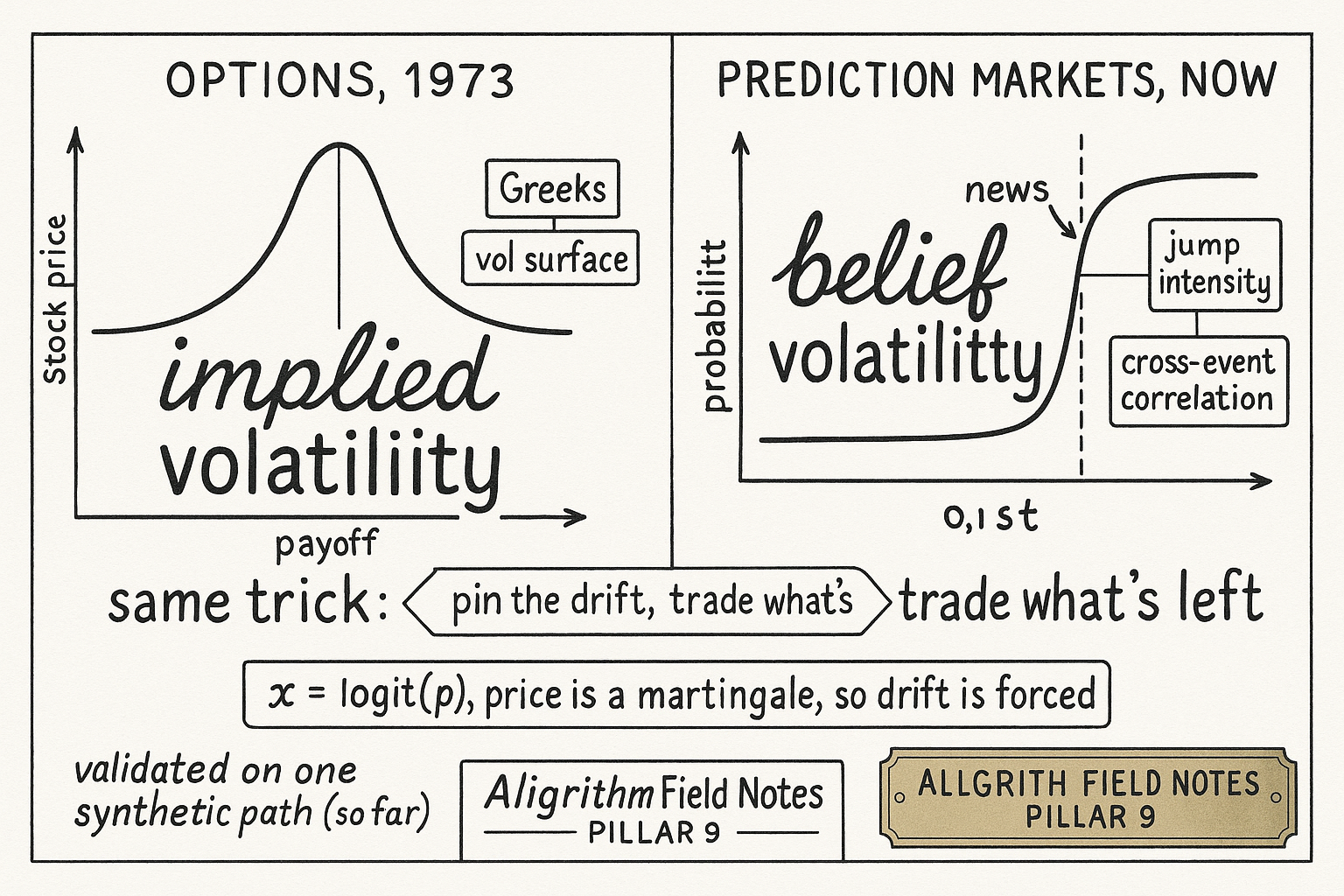
Options got a common language in 1973. Before Black-Scholes, a dealer quoting a call had to argue about the whole distribution of the stock at expiry. After it, everyone agreed to argue about one number, implied volatility, and hedge the rest with Greeks. The model was never "true." It coordinated a market around a small set of state variables, and that coordination is what let the options business scale into a derivative stack worth trillions.
Prediction markets have no such language. Polymarket, Kalshi and their cousins trade a contract that pays a dollar if an event happens and nothing if it doesn't, and the price sits in the open interval between zero and one so you can read it as a probability. But there is no shared model for how that probability should move through time, gap on news, or co-move with a related market. A recent paper from the Daedalus Research Team proposes to borrow the Black-Scholes trick wholesale: model the log-odds of the price as a jump-diffusion, force the price to be a martingale so the drift is not a free parameter, and whatever is left over becomes the tradable risk. This article walks through that kernel, the derivative layer it implies, and why the empirical case for it is thinner than the theory.
Trade the log-odds, not the probability
A probability is a bad state variable. It lives between zero and one, so a naive random walk will eventually push it through a boundary where it makes no sense, and its volatility has to shrink to nothing near the edges or the process escapes. The fix is the same one a softmax layer uses. Map the probability to its log-odds, run your dynamics on the unbounded line, and map back with a sigmoid.
$$ x_t = \operatorname{logit}(p_t) = \log \frac{p_t}{1-p_t}, \qquad p_t = S(x_t) = \frac{1}{1+e^{-x_t}} $$
The variable x is the log-odds, free to wander anywhere on the real line, and S is the logistic squashing function that pulls it back into a valid probability. Work a number: a price of p equal to 0.6 is x equal to log of 0.6 over 0.4, which is log 1.5, about 0.405. A price of 0.5 is x equal to zero. Push x out to 3 and p is about 0.95; push it to minus 3 and p is about 0.05. The same move in x buys you less and less probability as you approach the boundary, which is exactly the behavior you want.
If this map feels familiar it should. The old article "If You've Used a Softmax Layer, You Already Know the Price Formula" showed that the logistic and softmax are the same object the market maker uses to turn an unbounded score into normalized prices. This paper is running that map in reverse and then putting a stochastic process on the score.
The kernel is a jump-diffusion in log-odds
With x on the real line you can use the standard machinery. The paper writes belief dynamics as an Itô-Lévy process with three pieces: a drift, a diffusion, and a jump term.
$$ dx_t = \mu(t, x_t)\, dt + \sigma_b(t, x_t)\, dW_t + \int_{\mathbb{R}} z\, \tilde{N}(dt, dz) $$
Read the three pieces. The drift mu is the slow, predictable pull. The middle term is a Brownian motion scaled by sigma-b, the belief volatility, which is how fast log-odds wobble on ordinary order flow. The last term is the jump: a compensated random measure that lets the log-odds lurch by an amount z when news lands, rather than crawl there continuously. That third piece is the honest part of the model, because event prices really do gap. A court ruling drops, a candidate concedes, an economic print surprises, and the price teleports.
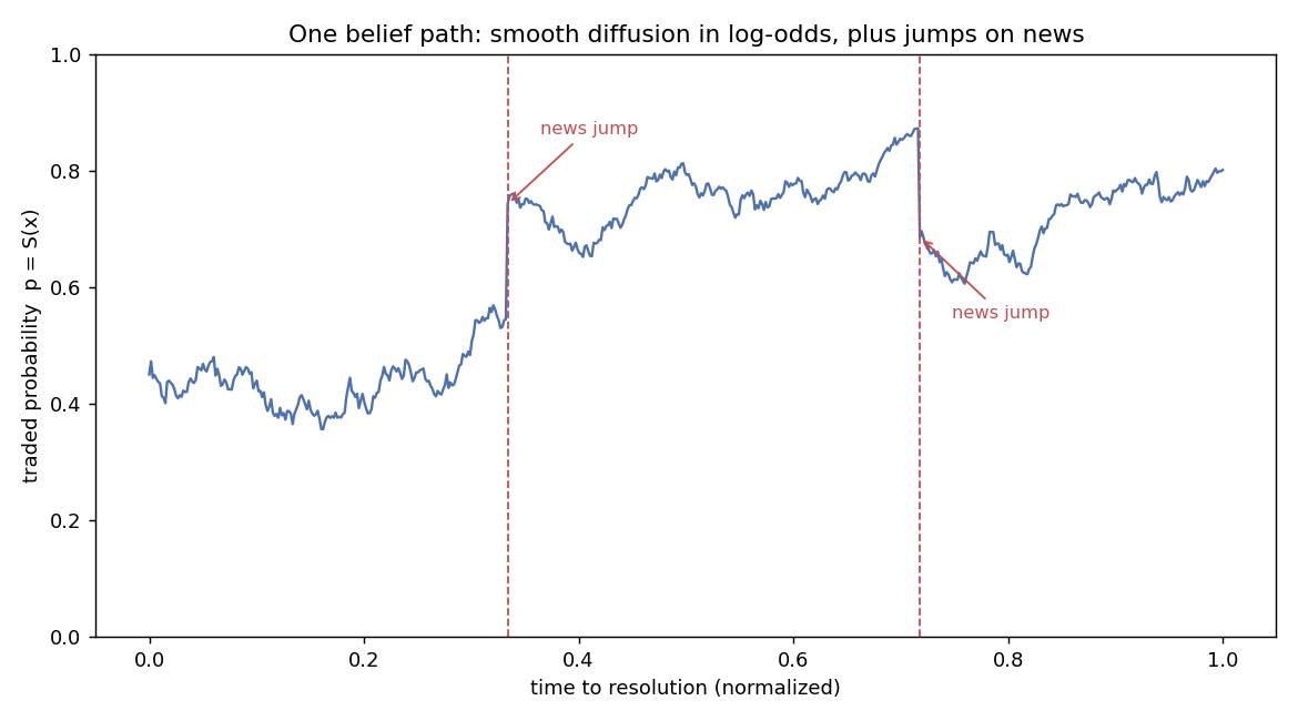
The figure is one simulated path. Between the dashed lines the probability grinds around on diffusion, and at each dashed line a jump snaps it to a new level in a single step. A market maker warehousing this contract is not mainly exposed to where the price ends up. They are exposed to the path: the wobble around the middle, and the gaps on announcements. That is the risk the rest of the framework is trying to make tradable.
The drift is not yours to choose
Here is the load-bearing idea, and it is the direct analogue of Black-Scholes. Because the price is the discounted risk-neutral value of a one-dollar payoff, it has to be a martingale: no expected drift under the pricing measure. But the log-odds map is nonlinear, so a zero-drift price does not mean a zero-drift x. Apply Itô's formula to the sigmoid and the convexity forces a specific drift on x.
$$ \mu(t,x) = -\,\frac{\tfrac{1}{2} S''(x)\, \sigma_b^2(t,x) + \int_{\mathbb{R}} \big( S(x+z) - S(x) - S'(x)\chi(z) \big)\, \nu_t(dz)}{S'(x)} $$
In words: the drift of the log-odds is whatever it has to be to cancel the curvature and jump-compensation terms, so that the probability itself has no expected change. Take the diffusion-only case with no jumps, where S-prime is p times one minus p and S-double-prime is that times one minus two-p. The drift collapses to minus one-half times one minus two-p times sigma-b squared. Plug in p equal to 0.6 and a belief vol of 0.8: the drift is minus one-half times minus 0.2 times 0.64, which is plus 0.064. The log-odds is nudged gently upward not because anyone thinks the event got likelier, but purely to offset the convexity of the sigmoid and keep the price a fair game.
This is the same discipline as the old article "Arbitrage Is Just Projection: One Calculation Gives Trade, Profit, and Target Prices." No-arbitrage is not a vibe, it is a constraint that pins down a specific quantity. There, projecting onto the no-arbitrage subspace gave you the trade and the target prices in one shot. Here, imposing the martingale property gives you the drift in one shot. Once the drift is spoken for, it stops being a knob. What remains free, and therefore what you can actually quote and hedge, is belief volatility, jump intensity and size, and cross-event correlation.
The derivative layer: sell spread, buy variance
If belief volatility is the free risk, you want to trade it directly instead of eating it through inventory. The options market solved this with variance and volatility swaps, and the paper transplants them. A belief-variance swap pays the realized quadratic variation of the log-odds against a fixed strike, and under slowly varying parameters that strike has a clean form.
$$ K_{t,T}^{x,\text{var}} \approx \int_t^T \sigma_b^2(u)\, du + \int_t^T \lambda(u)\, \mathbb{E}[z^2(u)]\, du $$
The fair strike is the sum of two variance sources: the diffusion part, the integral of belief vol squared, plus the jump part, the jump intensity lambda times the expected squared jump size. Work it over ten days. Say belief vol squared runs at 0.64 per day, so the diffusion piece is 6.4. Say jumps arrive at intensity 0.2 per day with expected squared size 0.25, so the jump piece is 0.2 times 0.25 times ten, which is 0.5. The strike is about 6.9. A maker who sells tight spreads and is therefore short realized variance can buy this swap to neutralize the exposure, and the split tells them how much of the premium is paying for ordinary wobble versus gap risk.
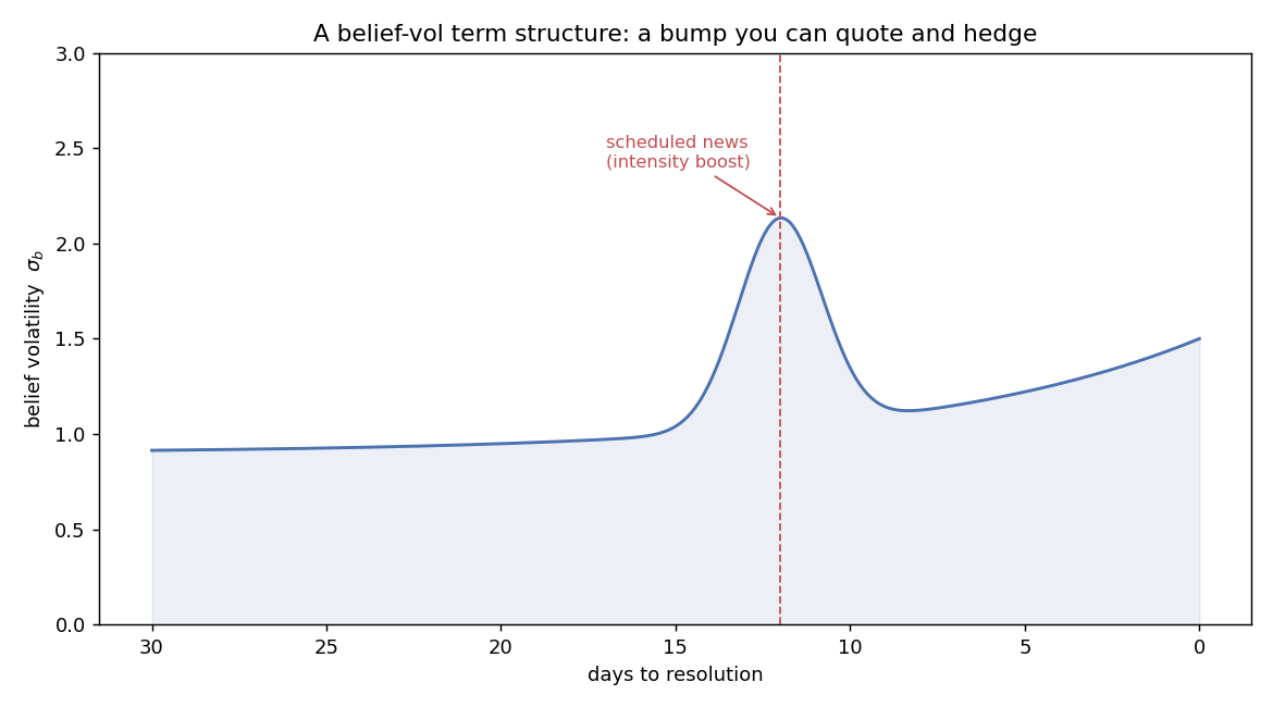
The strike is an integral over a belief-vol term structure, and that structure is not flat. The figure sketches the shape the paper wants you to calibrate: a baseline that rises into resolution as the outcome sharpens, plus a local bump on a scheduled announcement where you know intensity will spike. Once you can see that bump, you can budget your hedge for it, buying variance concentrated in the window where it actually accrues. The paper extends the menu with corridor variance, which only accrues while the price sits in a swing zone away from the boundaries, and correlation swaps that offset co-movement across related markets on something like an election night. Whether any venue will actually list these instruments is a separate question the paper does not answer.
Greeks that live in the middle of the board
To hedge any of this you need sensitivities, and in the log-odds parameterization they are almost embarrassingly simple. The delta and gamma of a vanilla contract with respect to x are just the first two derivatives of the sigmoid.
$$ \Delta_x = \frac{\partial p}{\partial x} = p(1-p), \qquad \Gamma_x = \frac{\partial^2 p}{\partial x^2} = p(1-p)(1-2p) $$
Delta is p times one minus p, which is maximized at 0.5 and dies at both boundaries. Gamma is that times one minus two-p, which is positive below the midpoint, zero at 0.5, and negative above it. Work the corners: at p equal to 0.5 delta is 0.25, its peak, and gamma is zero. At p equal to 0.9 delta is only 0.09 and gamma is 0.09 times minus 0.8, about minus 0.072. So a market pinned near 0.9 barely moves in probability terms even when the log-odds swings hard, while a coin-flip market at 0.5 has the most price sensitivity and the most dangerous curvature.
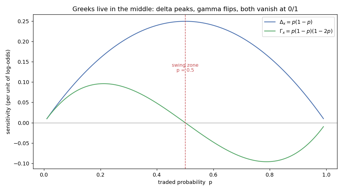
This is why liquidity and toxicity concentrate in the middle of the board. Order flow is most dangerous where gamma is largest and inventory turns fastest, which is the swing zone the corridor products target. The paper wraps this into an inventory-aware quoting rule, a version of the standard dealer reservation-price-and-spread recipe written in log-odds units, with the spread widening on toxic flow and pulling in near the boundaries where the contract barely moves. It is a sensible mapping, and it inherits the same limitation as every such rule: it is only as good as your estimate of belief vol.
Getting the numbers out of the tape
None of this is tradable without calibration, and the price you see is not the latent log-odds. It is that log-odds plus microstructure noise: stale quotes, bid-ask bounce, thin-book flicker. The paper's pipeline is a two-stage estimator. First a heteroskedastic state-space filter, a Kalman variant whose measurement noise is modeled as a function of spread, depth, trade rate and imbalance, recovers a smoothed latent log-odds from the noisy tape. Then an expectation-maximization step treats each log-odds increment as a mixture of a diffusion draw and a jump draw, and assigns each increment a posterior probability of being a jump. Increments that look like jumps get pulled out before estimating diffusion variance, so the belief-vol number is not contaminated by gaps. The refined variance and jump estimates feed the martingale drift formula, and one or two outer loops tighten it. The output is the belief-vol surface, a jump layer, and a dependence layer, indexed by time-to-resolution and moneyness.
The idea is coherent. Separate the signal from the noise, then separate the diffusion from the jumps, then enforce the no-arbitrage drift, and you get a stable object to quote off. The question is whether it actually forecasts better than something dumber.
Does it work? The evidence is one synthetic path
Here the paper gets thin, and honesty demands flagging it. The headline experiment is a single end-to-end forecast task: at each second, predict the realized log-odds variance over the next sixty seconds, then compare to what happened. The full model, RN-JD, is put up against a random walk in log-odds, a constant-volatility logit diffusion, a boundary-respecting Wright-Fisher diffusion, and an AR(1)-GARCH model, all evaluated causally on the same series.
| Model | MSE | MAE | QLIKE |
|---|---|---|---|
| RN-JD (this paper) | 70.28 | 1.588 | 1.462 |
| Random walk in logit | 77.41 | 1.163 | 4.732 |
| Constant-vol logit | 76.75 | 2.078 | 2.659 |
| Wright-Fisher (mapped) | 1.7e17 | 3.7e7 | 1.948 |
| AR(1)-GARCH (mapped) | 1.1e19 | 5.3e8 | 0.796 |
Read the table like a skeptic. RN-JD wins on squared and absolute error, which is the paper's claim. But the two probability-space baselines post error terms of ten-to-the-seventeenth and ten-to-the-nineteenth, which is not "worse," it is numerically detonating. When you map a GARCH forecast from probability space back to log-odds you divide by p times one minus p squared, and near a boundary that blows up. So most of RN-JD's MSE advantage is really a statement that its competitors explode when mapped, not that its variance forecast is sharp. Worse for the headline, on QLIKE, the loss that volatility researchers actually trust because it penalizes under-prediction and tolerates noise, the exploding AR(1)-GARCH still wins at 0.796 against RN-JD's 1.462. The paper's own preferred model loses on the metric its own field prefers.
And this is one path. The table is a single synthetic, risk-neutral-consistent simulation of six thousand steps, plus a mention of twenty Polymarket contracts that never turns into a real out-of-sample horse race. There is no cross-event calibration, no live A/B test, no confidence intervals. The paper is upfront that multi-event dependence and real deployment are future work. So take it for what it is: a well-constructed conceptual kernel with a proof-of-concept that does not yet clear the bar it sets for itself.
Why the idea might still matter
The paper's best argument is the one in its own conclusion: standardization beats realism. Black-Scholes coordinated options around implied vol despite being wrong about fat tails, jumps and stochastic volatility, all of which got bolted on later. What mattered was the shared vocabulary. If prediction markets are about to scale, and the ICE stake in Polymarket and billion-dollar monthly volumes suggest they are, then a common way to name belief volatility, jump intensity and cross-event correlation is worth more than any single forecast being accurate. The kernel's real contribution is not the sixty-second variance number. It is forcing the drift to be non-negotiable and exposing the remaining three factors as the things a desk should quote, hedge and eventually list swaps against.
Whether the market adopts that vocabulary is an empirical question the paper cannot settle from a synthetic path, and it would be a mistake to trade real inventory on this calibration as though it were validated. But as a map of what belief risk decomposes into, and where a maker's danger actually lives, the logit jump-diffusion is a clean and useful frame.
Where this connects
This kernel sits on top of two ideas this pillar has already built. The martingale drift is the same move as the old article "Arbitrage Is Just Projection: One Calculation Gives Trade, Profit, and Target Prices": no-arbitrage is a hard constraint that hands you a specific number rather than a vibe, and here the number is the drift of the log-odds. The logit map at the center is the object from the old article "If You've Used a Softmax Layer, You Already Know the Price Formula," run backward so you can put a stochastic process on the score and squash it into a valid price.
The market-maker layer connects forward to everything this pillar says about quoting under adverse selection. Belief vega, corridor variance and the swing-zone concentration of gamma are just precise names for where inventory hurts most, which is the same place tight spreads get picked off. The honest read is that the theory is ahead of the evidence. Treat the decomposition as a lens, not a live trading signal, until someone runs it out of sample on real multi-event data.
KEY POINTS
- Prediction markets lack the shared pricing language options got from Black-Scholes. The paper proposes the analogue: model the log-odds of the price as a jump-diffusion and standardize around belief volatility, jump intensity, and correlation.
- Trade the log-odds, not the probability. The logit map sends the bounded price to the whole real line where standard tools apply, and the sigmoid maps it back. It is the same map a softmax uses, run in reverse.
- The drift is not a free parameter. Forcing the price to be a martingale, the no-arbitrage condition, pins the log-odds drift to a convexity-plus-jump correction. In the diffusion-only case it is minus one-half times one minus two-p times belief vol squared.
- What is left free is what you can trade: belief volatility, jump size and intensity, and cross-event correlation. The paper defines variance swaps, corridor variance, and correlation swaps on these, with a fair variance strike that splits cleanly into a diffusion piece and a jump piece.
- The Greeks are trivial in log-odds units: delta is p times one minus p, gamma is that times one minus two-p. Delta peaks and gamma flips sign at 0.5, and both vanish at the boundaries, which is why toxicity concentrates in the swing zone.
- Calibration is a state-space filter to strip microstructure noise, then an EM step to separate diffusion from jumps, then enforcement of the martingale drift, yielding a belief-vol surface.
- The evidence is weak. The headline result is one synthetic path where the model wins on MSE mostly because its baselines numerically explode when mapped, and it loses on QLIKE, the metric volatility researchers prefer. Treat the kernel as a useful frame, not a validated trading signal.
A note on AI. The ideas, research, analysis, and conclusions in this article are my own. I use AI tools to help with editing and wordsmithing, because English is not my first language, and I am not shy about that. AI-generated ideas and AI-assisted writing are not the same thing: the first is empty slop from a generic prompt, the second is a tool for communicating years of real research more clearly. Judge the work by its substance, not by whether software helped polish the prose.