9. Prediction Market Arbitrage July 2, 2026 7 min

9.24 If You've Used a Softmax Layer, You Already Know the Price Formula

Softmax is the Polymarket price formula. Work one trade to the cent, see why the maker's loss is capped, why the liquidity parameter b sets price impact, and why arbitrage distance is measured in KL, not Euclidean.

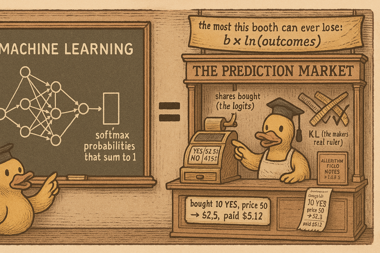
Train a classifier and you have already written the Polymarket pricing engine. The layer that turns raw network outputs into class probabilities, softmax, is the exact function a logarithmic market-scoring-rule maker uses to turn accumulated trades into prices. Same formula, same math, different bank account. The gateway article "Convex Geometry for Traders" said this in one line to keep you moving; this is the full derivation, with the numbers worked out, so you can read a market maker as a softmax layer with money on the line and know exactly why prices move the way they do.

The whole point of pinning down the pricing function is that every structural result in the pillar rides on it. The projection in "Arbitrage Is Just Projection" measures profit in a distance defined by this cost function. The solver crashes in "Why Your Arbitrage Solver Crashes at 99 Cents" because of this function's curvature at the boundary. Get the price formula concrete and those results stop being abstract.

Proper scoring rules: why truth is the profit-maximizing report

Start one level below prices, at the incentive. A scoring rule pays a forecaster based on the probability they report and the outcome that happens. It is proper when reporting your true belief maximizes your expected score, so honesty is not a virtue you hope for, it is the strategy that pays best.

$$ \mathbb{E}_q\bigl[S(q, \omega)\bigr] \;\ge\; \mathbb{E}_q\bigl[S(p, \omega)\bigr] \quad \text{for all } p \neq q $$

Read that as: if your true belief is q, then scoring yourself with your honest q gives at least as much expected score as reporting any other p. Two rules matter. The log score pays the log of the probability you assigned to what actually happened, and it is the seed of the market maker below. The quadratic, or Brier, score pays based on squared error and decomposes into calibration, discrimination, and base-rate uncertainty, which is the same decomposition the article "What a Market Price Actually Is" uses to gate informational trading. Every proper scoring rule converts into a market-maker cost function through one transform, so the maker's pricing inherits the honesty incentive of the rule it came from.

The cost function and the softmax price

The logarithmic market-scoring-rule maker, the one Polymarket and its kin use, holds a state vector, the running count of how many shares of each outcome have been bought. It sets a cost for reaching any state, and the price of each outcome is how fast that cost rises as you buy more of it.

$$ C(\theta) = b \, \ln\!\left( \sum_i \exp(\theta_i / b) \right), \qquad p_i(\theta) = \frac{\exp(\theta_i / b)}{\sum_j \exp(\theta_j / b)} $$

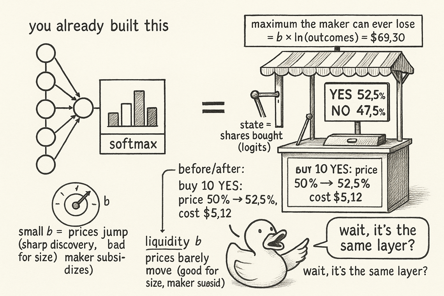
Read the left formula as: the cost of a state is a smoothed maximum of the state coordinates, scaled by a liquidity parameter b. Read the right as: the price of outcome i is the softmax of the state, e raised to that coordinate over b, divided by the sum so all prices are positive and sum to one. The state plays the role of logits, the prices are the softmax output, and buying delta shares of outcome i adds delta to that coordinate, which pushes its price up and drags every other price down because they must still sum to one. A machine-learning reader arrives fluent. This is also the substrate the article "Bayesian Edge in Log-Odds" leans on, because the state is a log-odds vector and updating a belief is adding a number to a coordinate, the same act as trading.

A trade, worked to the cent

Take a binary YES-NO market with liquidity parameter b equal to 100 and a fresh state of zero shares on each side. Both coordinates are zero, so the softmax gives each side e-to-the-zero over two e-to-the-zeros, which is 0.50. Fair coin, as it should be on an untouched market.

Now a trader buys 10 YES shares. The state becomes 10 on YES, 0 on NO. The new YES price is e-to-the-0.1 over the quantity e-to-the-0.1 plus 1, roughly 1.105 over 2.105, about 0.525. The price moved from 50 percent to 52.5 percent. What did that cost? The cost of the trade is the cost at the new state minus the cost at the old state.

$$ C(10, 0) - C(0, 0) = 100 \ln\!\left(e^{0.1} + 1\right) - 100 \ln 2 \approx 100\,(0.744 - 0.693) = \$5.12 $$

Read that as: buying 10 YES shares that will pay $10 if YES resolves true cost $5.12 and moved the market 2.5 points. The maker did not consult a forecast or a news feed. It ran the cost function, charged the integral of the price over the shares you bought, and updated the state. That is the entire pricing act.

Bounded loss and the meaning of b

Two properties make this maker safe to run and tunable to your market.

The maker's worst-case loss is bounded, and the bound is b times the log of the number of outcomes. For a binary market that is b times the log of 2, about 0.693 times b. At b equal to 100 the maker cannot lose more than $69.30 no matter how many trades cross, no matter who is right. That bound is why "The Market Maker's Impossibility" can argue the platform tolerates arbitrage: the downside is capped by construction.

The liquidity parameter b is the one knob, and it sets the tradeoff between price sensitivity and depth.

$$ \Delta p_i \;\approx\; \delta \, \frac{p_i \, (1 - p_i)}{b} $$

Read that as: the price impact of buying delta units of outcome i is roughly delta times p times one-minus-p, divided by b. Small b, say 10, means prices lurch on small orders, good for fast price discovery and brutal for anyone trying to fill size. Large b, say 1,000, means the book barely moves, good for large orders and expensive for the maker who is subsidizing that depth. The impact is largest at a price of 0.50, where p times one-minus-p peaks, and it vanishes as the price approaches 0 or 1. That last fact is the seed of a problem: near the boundary the price barely moves per share on the way in, but the curvature of the cost function explodes, which is precisely the gradient blow-up that forces Barrier Frank-Wolfe in "Why Your Arbitrage Solver Crashes at 99 Cents."

Two coordinate systems, and why a trader needs both

A market has two honest descriptions, and you need to move between them. The state space counts shares, unbounded, where a trade is just addition. The price space shows probabilities, bounded in zero to one, summing to one, which is what the screen displays. The convex conjugate, the Legendre-Fenchel transform, is the translator.

$$ \theta \to p: \; p = \nabla C(\theta) \quad (\text{softmax}), \qquad p \to \theta: \; \theta = \nabla R^*(p) \quad (\text{log}) $$

Read that as: apply the gradient of the cost function to a state and you get prices, the softmax direction; apply the gradient of the conjugate to prices and you get back the state, the log direction. For this maker the conjugate is negative entropy scaled by b, the sum of p-i times log p-i. You need the log direction for one concrete reason. The arbitrage math in "Arbitrage Is Just Projection" hands you target prices, the fair vector the market should show, but an exchange only accepts orders in shares. The optimal trade is the gradient of the conjugate at the target prices minus your current state, which is the log-direction map turning "the market should be priced here" into "buy this many of these contracts." Skip the conjugate and you have a target you cannot place.

The curved ruler: Bregman and KL

Distance in this market is not Euclidean, and using the wrong ruler costs money. The Bregman divergence built from the cost function is the honest measure.

$$ D_R(p \,\|\, q) = R(p) - R(q) - \nabla R(q) \cdot (p - q) $$

Read that as: take the value of the convex function R at p, subtract its value at q, then subtract the tangent-line approximation of R at q evaluated at p; what is left is the gap between the true curve and its tangent, a distance that respects the function's curvature. Plug in negative entropy, the conjugate of this maker's cost, and the divergence collapses to KL divergence, the sum of p-i times log of p-i over q-i. Plug in one-half the squared norm and it collapses to plain Euclidean distance. The maker measures in KL because the maker's cost function is built on the log score, so the guaranteed arbitrage profit in the projection theorem is a KL distance from the current prices to the fair set. The old article "Entropy as a Market Concept" builds the intuition for why entropy and its divergences are the natural language of an information market, and this is that idea made into a pricing engine.

KEY POINTS

The logarithmic market-scoring-rule maker prices with softmax. The state vector is the logits, the prices are the softmax output, and buying shares adds to a coordinate and pushes that price up. If you have used softmax, you know the price formula.
Proper scoring rules pay most for honest reports; the log score seeds this maker, the Brier score gives the calibration decomposition. Every proper scoring rule becomes a cost function through the Legendre-Fenchel transform.
Worked trade: binary market, b equal to 100, buy 10 YES shares, price moves 50 percent to 52.5 percent and costs $5.12. The maker runs the cost function, charges the integral of price over shares, and updates the state. No forecast involved.
The maker's worst-case loss is bounded at b times the log of the outcome count, about $69.30 for a binary market at b equal to 100. This bound is why the platform can tolerate arbitrage.
The liquidity parameter b sets sensitivity against depth. Price impact is roughly delta times p times one-minus-p over b, largest at 0.50 and vanishing near 0 and 1. That boundary behavior is the seed of the solver blow-up that forces Barrier Frank-Wolfe.
The convex conjugate translates between shares and prices: softmax one way, log the other. You need the log direction to convert the arbitrage math's target prices into actual share orders.
Distance in this market is KL, not Euclidean, because the cost is built on the log score. The Bregman divergence from negative entropy is KL, and it is the ruler the projection theorem measures guaranteed profit with.

References

- Elicitation of Personal Probabilities and Expectations - Savage (1971)
- Verification of Forecasts Expressed in Terms of Probability - Brier (1950)
- An Optimization-Based Framework for Automated Market-Making - Abernethy et al. (2011)
- Logarithmic Market Scoring Rules for Modular Combinatorial Information Aggregation - Hanson (2007)
- Convex Optimization - Boyd and Vandenberghe (2004)
- The Relaxation Method of Finding the Common Point of Convex Sets - Bregman (1967)