6.55 Piecewise-Linear Regime Identification (Interpretable, No Black Box)
Piecewise-linear regime detection on the Swiss SLI reports in-sample R-squared 0.954 at 15 breakpoints. A driftless random walk scores 0.966, and the knee sits on an optimizer failure.

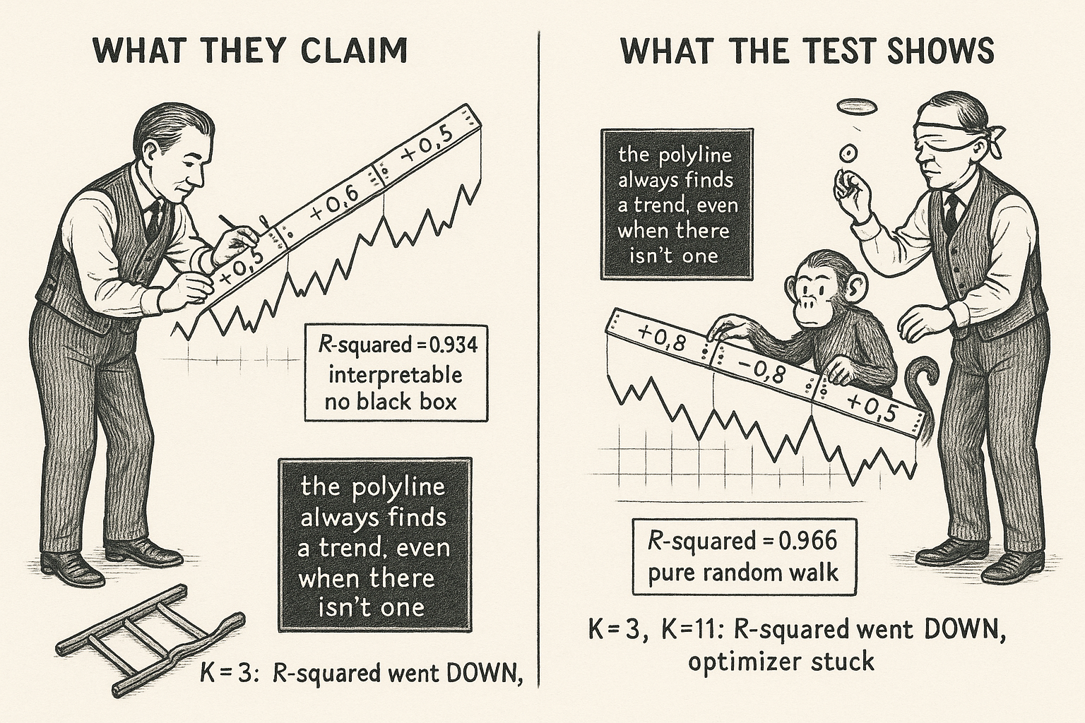
Fit a connected piecewise-linear trend to the Swiss Leaders Index with fifteen breakpoints and you get an in-sample R-squared of 0.954. Fit the same model to a driftless random walk of the same length and you get 0.966. I ran 200 of them. The noise wins at every single value of K, from zero breakpoints to fifteen. Whatever the 0.954 is measuring, it is not evidence that the SLI has regimes.
This research note from Andreas Steiner Consulting proposes segmented regression as an interpretable substitute for black-box regime models: fit straight lines joined end to end, optimize the joint locations, pick the number of joints by the elbow of the R-squared curve, and read off a bullish or bearish label from each segment's slope. The machinery is clean and the presentation is honest about being descriptive. The problem is what happens between the equations and the chart. Their own reported R-squared ladder violates a property that nested least-squares fits cannot violate, and the breakpoint count they ship sits exactly on top of that violation.
Start with what the model is, because the paper's own Section on splines gives away more than it intends.
The model is a one-layer ReLU network wearing a suit
Standard linear regression on a time index assumes one slope for the whole sample. Segmented regression relaxes that by letting the slope change at K locations. Enforcing continuity at those locations, which the paper does and which matters because a jumping fitted price is nonsense, gives the truncated power form.
$$ y_t = \beta_0 + \beta_1 t + \sum_{j=1}^{K} \beta_{j+1}\,(t-\tau_j)_+ + \epsilon_t, \qquad (x)_+ = \max(0,x) $$ $$ \text{slope on segment } m \;=\; \beta_1 + \sum_{j=1}^{m-1}\beta_{j+1} $$
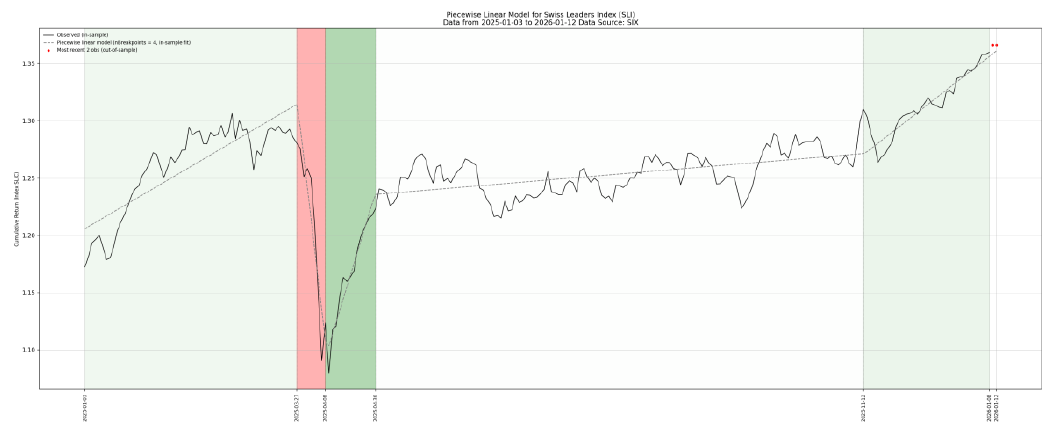
The hinge term contributes nothing before its breakpoint and grows linearly after it, so beta-sub-(j+1) is the change in slope at breakpoint tau-sub-j, and the slope on any segment is the starting slope plus every change that has already fired. Worked example using the four-breakpoint SLI fit, with coefficients I reconstructed by reading levels and dates off the paper's own chart (the paper prints no coefficient table, so treat these as my reconstruction, not their output). Take beta-0 = 1.205 and beta-1 = 0.00184 index units per day, with breakpoints at trading days 58, 66, 91 and 216, which map to 27 March 2025, 8 April 2025, 14 May 2025 and 11 November 2025. Set beta-2 = -0.02144, beta-3 = +0.02292, beta-4 = -0.00310 and beta-5 = +0.00092.
Segment 1 runs at 0.00184 per day and carries the index from 1.205 to 1.205 + 58(0.00184) = 1.3117 by 27 March. Segment 2 runs at 0.00184 - 0.02144 = -0.01960 per day, so over the eight days into 8 April the index falls to 1.3117 - 8(0.01960) = 1.1549, a 12% drawdown. Segment 3 runs at -0.01960 + 0.02292 = +0.00332, recovering to 1.1549 + 25(0.00332) = 1.2379 by 14 May. Segment 4 runs at +0.00022, which over 125 trading days moves the index to 1.2654 and is a flat line with extra steps. Segment 5 runs at +0.00114 and closes at 1.3133. Those five endpoint levels match the fitted dashed line in the paper's chart to within the width of the line.
Now look at what that equation actually is. Input t, K hidden units of the form max(0, t minus a bias), a linear skip connection, and a linear output layer. That is a one-hidden-layer ReLU network with the input weights frozen at one, and fitting it means solving OLS for the output layer while running a quasi-Newton optimizer on the hidden biases. The paper's title claim of no black box rests on the network being tiny and the plot being legible, which is a fair reason to prefer it. It is not a different species of model, and it inherits the training pathologies of the species it belongs to. Hold that thought, because those pathologies show up in their results table.
Locating the breakpoints, and why L-BFGS-B was the wrong hammer
With K fixed, the coefficients come from OLS in closed form, so the only hard part is the breakpoint positions. The paper concentrates the coefficients out and minimizes the residual sum of squares over the knot vector.
$$ \min_{\tau_1,\dots,\tau_K}\ \mathrm{RSS}(\tau)=\sum_{t=1}^{T}\bigl(y_t-\hat y_t(\tau)\bigr)^2 \qquad \text{s.t.}\quad \tau_{\min}<\tau_1<\tau_2<\cdots<\tau_K<\tau_{\max} $$
Read it as: slide the joints around until the fitted polyline hugs the data as tightly as possible, keeping the joints in order and keeping a minimum number of observations inside each segment. The paper uses L-BFGS-B, a quasi-Newton method with box constraints, initialized at equally spaced knots, and enforces the ordering by sorting inside the loop. Worked scale: with T of about 255 daily observations, the number of distinct knot configurations at K=4 is 254-choose-4, which is 169,362,501. At K=15 it is 254-choose-15, about 5.9 times 10 to the 23. The paper calls exhaustive search infeasible and it is right about K=15. It is wrong about K=4, and K=4 is the model they ship. On a laptop with rank-one residual updates, 169 million configurations is an overnight job at worst.
Two things make L-BFGS-B a poor fit here, and both are visible in the output. First, the profiled RSS is continuous in tau but kinked at every integer, because moving a knot past a data point changes which observations that hinge column touches. Quasi-Newton methods build a curvature estimate that assumes smoothness, and on a kinked surface the curvature estimate is garbage near the kinks. Second, sorting the knots inside the objective makes the function non-differentiable wherever two knots cross, which corrupts the same curvature estimate a second time. Add the dead-unit failure mode from the network view: if a knot wanders past the end of the sample, its hinge column becomes all zeros, its gradient becomes exactly zero, and it never comes back.
Their own R-squared ladder proves the optimizer failed
Here is the check that takes thirty seconds and that nobody ran. Piecewise-linear models are nested in the number of breakpoints. Any K-breakpoint solution is reachable from a (K+1)-breakpoint model by setting the extra slope change to zero or by stacking two knots on the same date. So at the global optimum, R-squared must be non-decreasing in K. It cannot go down. Ever.
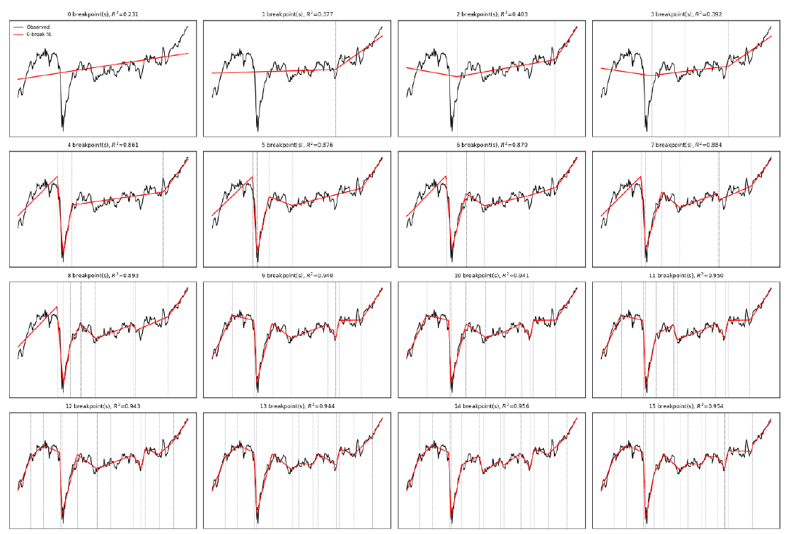
Read the R-squared values off the panel titles: 0.231, 0.377, 0.403, 0.392, 0.861, 0.876, 0.879, 0.884, 0.893, 0.940, 0.941, 0.930, 0.943, 0.944, 0.956, 0.954. It goes down three times. K=3 scores 0.392 against K=2's 0.403. K=11 scores 0.930 against K=10's 0.941. And K=15, the headline number in the abstract, scores 0.954 against K=14's 0.956. Three violations out of fifteen steps. Each one is a proof that the optimizer returned a local minimum rather than the global one, and the K=3 failure is the largest of the three.
I am not correcting these numbers. They are what the source reports, and the source may simply be wrong about them. What I will say is that the reported ladder and the stated method are inconsistent with each other, and the paper does not flag it.
The knee is a real algorithm sitting on a broken input
The elbow rule is the paper's answer to model selection, and the algorithm itself is fine. Draw the chord from the first point of the R-squared curve to the last, then take the point with the largest perpendicular distance above it.
$$ R^2(K)=1-\frac{\mathrm{RSS}(K)}{\mathrm{SS}_{\mathrm{tot}}},\qquad \mathbf{v}=\bigl[K_{\max}-0,\ R^2(K_{\max})-R^2(0)\bigr] $$ $$ d_k=\frac{\bigl|\,v_x\bigl(R^2(k)-R^2(0)\bigr)-v_y\,k\,\bigr|}{\|\mathbf{v}\|}, \qquad k^{*}=\arg\max_k d_k $$
The numerator is a two-dimensional cross product measuring how far the curve bulges above the straight line, and the denominator rescales it into a distance. Worked example on the paper's own ladder. The chord runs from (0, 0.231) to (15, 0.954), so v = [15, 0.723] and the norm of v is 15.017. At k=4 the numerator is 15(0.861 - 0.231) - 0.723(4) = 9.450 - 2.892 = 6.558, giving d = 0.4367. At k=5 it is 15(0.876 - 0.231) - 0.723(5) = 6.060, giving 0.4035. At k=9 it is 4.128, giving 0.2749. The maximum sits at k=4 with 0.4367, which reproduces the red dot in their figure exactly.
Two observations. The norm of v is the same constant for every k, so dividing by it changes nothing about which k wins. Strip it out and the knee is just the point of maximum vertical gap above the chord, and at k=4 that gap is 6.558 divided by 15, or 0.437 of R-squared. The perpendicular framing is decoration.
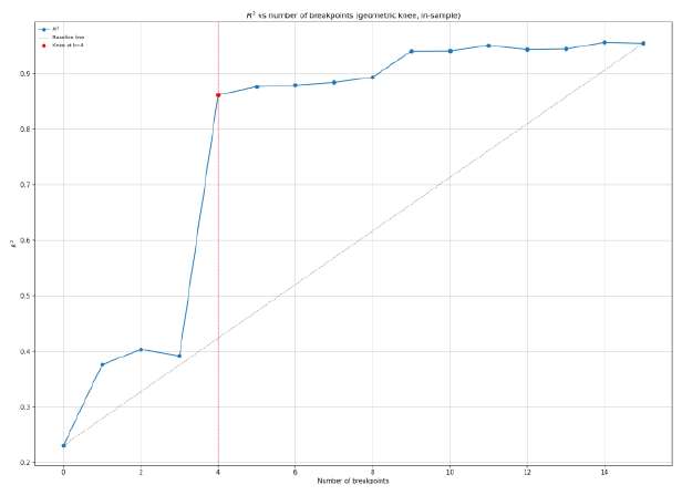
The second observation is the damaging one. K=4 wins the knee contest by a wide margin because of the vertical cliff from 0.392 to 0.861 between K=3 and K=4, and that cliff is partly an artifact of the K=3 optimization failure. Part of the jump is real: the March-April crash is a V, and a V needs two knots to model, so no three-knot fit can be as good as a four-knot one. But the reported K=3 value of 0.392 is provably not the global optimum, since 0.403 is achievable by construction. If the true K=3 optimum lands anywhere near 0.8, and a rally-crash-rebound-drift configuration with three knots is available in the data, the cliff shrinks and the knee moves or disappears. The knee inherits every error in the curve it reads.
Why they needed the knee in the first place
The paper lists AIC and BIC before reaching for the elbow, then drops them without showing the numbers. Run them. With T = 253 and RSS proportional to one minus R-squared, moving from K=4 to K=15 changes the goodness-of-fit term by T times the log of (1 - 0.954) over (1 - 0.861), which is 253 times the log of 0.3309, or -279.8. The AIC penalty as the paper writes it, 2(K+2), rises by only 22 over the same interval. The BIC penalty, (K+2) log T with log 253 = 5.5334, rises by 60.9. Both criteria pick K=15 by a margin of more than 200 units.
It gets worse under an honest parameter count. The paper counts K+2 coefficients and ignores the K breakpoint locations, which are estimated from the same data and cost degrees of freedom. Count 2K+2 and the AIC penalty gap becomes 44 and the BIC gap becomes 121.7. Still nowhere near 279.8. Zhang and Siegmund built a modified BIC for precisely this undercount, and the paper cites it as reference [3] without using it.
So AIC and BIC both run away to the maximum complexity the analyst allows, the analyst does not want fifteen regimes on one year of data, and the knee delivers four. That is the actual sequence. It is a defensible piece of judgment and the paper should present it as judgment rather than as a third selection criterion sitting alongside the other two.
Noise fits better than the SLI does
Here is the test that settles whether any of this R-squared is informative. I generated 200 driftless random walks of 253 observations, fitted connected piecewise-linear models with K from 0 to 15 by greedy forward knot selection on an integer grid, and recorded the in-sample R-squared. R-squared is scale invariant for a driftless random walk, so the daily volatility does not enter and there is nothing to tune.
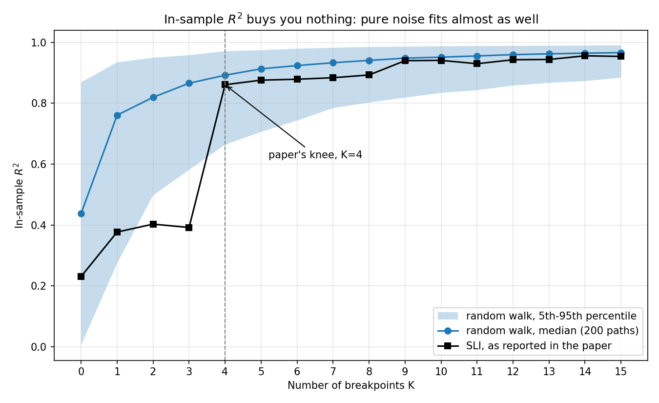
Median random-walk R-squared: 0.438 at K=0, 0.892 at K=4, 0.966 at K=15. The SLI: 0.231, 0.861, 0.954. Pure noise beats the real index at every breakpoint count. The comparison is generous to the paper, because greedy selection on a coarse integer grid is a weaker optimizer than continuous L-BFGS-B, so the null numbers are a floor rather than a ceiling.
None of this says the SLI lacked structure in 2025. It says in-sample R-squared on a price level cannot tell you whether it did. A random walk is locally trending everywhere, so a polyline with free knots will always find trends in it, and the number it reports back is a measure of how many knots you granted, not of how regime-like the series is. The paper reports 0.954 as a headline. It is the least informative number in the note.
The regime labels are arithmetic, not estimation
The final step assigns each segment a label from its slope, and the paper estimates that slope by regressing the fitted values on time within the segment.
$$ \hat\beta_{\text{seg}}=\frac{\sum_{t=s}^{e}(t-\bar t)\,\hat y_t}{\sum_{t=s}^{e}(t-\bar t)^2}, \qquad \bar t=\frac{s+e}{2} $$ $$ \text{label}=\begin{cases}\text{bullish} & \hat\beta_{\text{seg}}>\theta\\[2pt] \text{bearish} & \hat\beta_{\text{seg}}<-\theta\\[2pt] \text{consolidation} & |\hat\beta_{\text{seg}}|\le\theta\end{cases} \qquad \theta=\text{66th pct of }\{\hat\beta_{\text{seg}}\} $$
The regression is a no-op. Inside a segment the fitted values are exactly a straight line by construction, so OLS of y-hat on t returns that line's slope with an R-squared of one and recovers beta-1 plus the accumulated slope changes to machine precision. Running a regression here dresses up a subtraction.
The threshold is worse. Worked example on the five SLI segments, using the slopes reconstructed above: -0.01960, +0.00022, +0.00114, +0.00184, +0.00332. Sorted, the 66th percentile by linear interpolation sits at position 0.66 times 4 = 2.64, between 0.00114 and 0.00184, giving theta = 0.001588. Apply it: segments 1 and 3 come out bullish, segment 2 bearish, segments 4 and 5 consolidation. Change nothing about the market and set theta at the 50th percentile instead and segment 5 flips to bullish. A percentile threshold on five numbers does not classify market states, it partitions a five-element list into buckets whose sizes you chose in advance. With K=4 you will get roughly 1.7 bullish segments no matter what the index did.
What it is good for, and what it cannot do
The fatal constraint for anyone thinking about trading this: the breakpoints are located using the whole sample. That last knot on 11 November 2025 was placed knowing what happened through 12 January 2026. On 11 November itself, with no future data, the optimizer has no reason to put a knot there. The paper's chart legend holds out two observations as out-of-sample. Two. The knee, the breakpoint count and every knot position come from the full history.
That gap is the whole difference between this and a state-space regime model. The old article "Regime-Switching That Works, Factors That Don't (MS-GARCH)" covers the alternative: a Markov-switching specification gives you a transition matrix and a filtered probability of being in each state using information available at time t, which is a number you can size a position with. Segmented regression gives you a retrospective annotation. Both are called regime detection and only one of them runs forward.
Used inside its actual range, the method earns its place. As a compression device it is excellent: five slopes and four dates summarize a year of daily prices in a form a risk committee can read without a tutorial, and the paper's stated applications of conditioning performance attribution and factor exposures on identified periods are legitimate ex-post analysis where hindsight is allowed. The extensions the paper sketches are the right ones, particularly robust loss functions in place of OLS, since a single crash segment of eight observations carries enormous leverage on the squared-error objective. Warwicker and Rebennack solve exactly the robust continuous piecewise-linear problem to global optimality with a Benders decomposition, which would also fix the local-minimum failures shown above. Muggeo's iterative linearization would at least give standard errors on the breakpoint dates, which the paper does not report and which would immediately show how loosely the 14 May knot is pinned down.
The verdict: correct model, honest framing of its purpose, and a validation section that measures nothing. Report the segment slopes and dates. Delete the R-squared.
KEY POINTS
- The connected piecewise-linear model is a truncated power spline with free knots, which is identical to a one-hidden-layer ReLU network with unit input weights and a linear skip. Calling it "no black box" describes the size of the plot, not a difference in kind, and the model inherits the same training pathologies.
- The paper's own R-squared ladder decreases three times as breakpoints are added: 0.403 to 0.392 at K=3, 0.941 to 0.930 at K=11, and 0.956 to 0.954 at K=15. Nested least-squares fits cannot do that at the global optimum, so L-BFGS-B returned local minima. The source reports these numbers without flagging the contradiction.
- The geometric knee reproduces at K=4 (perpendicular distance 0.4367 against 0.4035 at K=5), but it wins on the 0.392-to-0.861 cliff, and the 0.392 endpoint of that cliff is the largest of the three optimizer failures. Fix K=3 and the knee may move.
- AIC and BIC both select K=15 by more than 200 units, even after correcting the paper's parameter count from K+2 to 2K+2. The knee is the analyst overruling both criteria, which is reasonable, and should be labelled as judgment rather than as a third criterion.
- Across 200 driftless random walks of 253 observations, median in-sample R-squared is 0.892 at K=4 and 0.966 at K=15, above the SLI's 0.861 and 0.954 at every K. In-sample R-squared on a price level measures knot count, not regime structure.
- Regressing fitted values on time inside a segment recovers the segment slope exactly and adds nothing. A 66th-percentile threshold applied to five slopes fixes the number of bullish segments before looking at the market.
- Every breakpoint is placed with full-sample hindsight and the paper holds out two observations. Use this to summarize history and condition attribution after the fact. For a signal that runs forward, you need filtered state probabilities, not a retrospective polyline.