6.54 Volatility Clustering in Bitcoin: Regime Persistence as a Forecast
Bitcoin vol clustering: a 3-state Markov chain shows persistence above 0.9 -- High state delivers ~9% moves in 48h, but thresholds are look-ahead by construction.
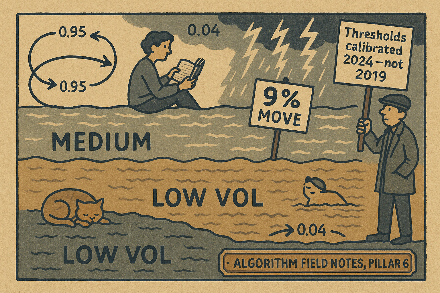
Bitcoin's volatility does not mix randomly across time. High-vol periods follow high-vol periods, low-vol stretches extend themselves, and the transition probabilities are stable enough to build a forecast from. Borrego Roldán's 2024 study quantifies this with hourly and daily data from August 2018 to November 2024, constructing 3-state Markov chains around rolling log-volatility and checking whether knowing today's regime tells you anything about tomorrow's moves. It does. But the infrastructure underneath carries a problem worth understanding before you act on any of it.
How you measure the thing in the first place
The study computes rolling historical volatility the standard way: standard deviation of returns over a trailing window. Returns are price ratios, not log returns.
$$ R_t = \frac{O_t}{O_{t-1}}, \qquad \sigma_t = \text{std}(R_{t-n+1}, \ldots, R_t) $$
O is the open price at time t, and n is the window length. The author then takes the natural log of that series.
$$ LV_t = \ln(\sigma_t) $$
Worked example: suppose the last 24 hourly returns have a standard deviation of 0.003 (0.3% per hour). Log-volatility at that point is ln(0.003) = -5.81. A more turbulent stretch with std 0.008 gives ln(0.008) = -4.82. The logged series is stationary across almost all windows tested, with ADF p-values well below 0.01. The exception is the 90-day daily window, which required differencing. Everything below uses log-volatility.
The paper runs this across five timeframes (1h, 4h, 6h, 12h, 1d) and multiple window sizes in each. Autocorrelation functions confirm the clustering: for 1h data with a 24-period window, the ACF at lag 24 sits around 0.65. The lag at which autocorrelation becomes statistically insignificant roughly corresponds to the window length itself. Short windows cluster fast and go quiet fast; longer windows carry structure out to larger lags.
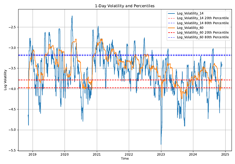
Look at how long vol stays above the 80th percentile band (the upper dashed line) versus how rarely it crosses between bands in a single day. That is the clustering, made visible. Also notice the problem: the bands are fixed horizontal lines, computed from the full 2019-2025 history. From 2019's vantage point those lines did not exist yet.
Carving the series into three states
Three states are enough: Low (below the 20th percentile of log-volatility over the full sample), Medium (between the 20th and 80th), and High (above the 80th). With the 1h, 24-period window those thresholds are fixed numbers. Each hour, the current log-vol drops into one of the three buckets.
$$ \text{State}_t = \begin{cases} 1 & \text{if } LV_t < P_{20} \\ 2 & \text{if } P_{20} \le LV_t \le P_{80} \\ 3 & \text{if } LV_t > P_{80} \end{cases} $$
Worked: P20 = -5.0, P80 = -4.4 (illustrative values; the actual cutoffs depend on the window and timeframe). A current LV of -5.5 goes into State 1; LV of -4.7 goes into State 2; LV of -4.0 goes into State 3. From there the analysis asks: given you are in State i right now, what is the probability you are in State j one period later?
The Markov numbers
The transitions are estimated by counting: out of all the hours where vol was in State 1, what fraction transitioned to State 1, State 2, or State 3 the next hour? That gives one row of the matrix. Repeat for all three states.
$$ P_{ij} = \Pr(\text{State}_{t+1} = j \mid \text{State}_t = i), \qquad \sum_j P_{ij} = 1 $$
P sub ij is the probability of moving from state i to state j. Each row sums to 1. The diagonal entries are what matter here: they are the persistence probabilities, the chance of staying in the same state.
For 1h data with a 24-period vol window:
| State | Stay in state | Leak to Medium | Leak to other |
|---|---|---|---|
| Low | 0.9505 | 0.0488 | 0.0007 |
| Med | 0.9715 | (own state) | 0.0164 / 0.0121 |
| High | 0.9629 | 0.0369 | 0.0003 |
With a 48-period window the persistence rises further: Low stays at 0.975, Medium at 0.985, High at 0.980. Widen the window and the state becomes stickier, because a 48-hour rolling std does not shake off a single noisy hour. Cross to the daily timeframe with a 7-period window and you get the lowest persistence in the whole study: the Low state stays at only 0.8167. That is the floor. Still above 80%, but meaningfully lower than the hourly figures. By the time you use a 90-period daily window, persistence climbs back to 0.9705/0.9819/0.9774 across the three states.
Worked interpretation of the 1h, 24-period matrix: you are in the Low vol state. Tomorrow's probability distribution across states is 95.05% Low, 4.88% Medium, 0.07% High. The direct transition from Low to High in a single step is essentially zero. To reach High, vol has to transit through Medium first, which takes multiple steps. That is the clustering in matrix form.
What each state predicts about moves
This is the part that has a trading application. For each vol state, the paper measures subsequent absolute price moves over standardized lookahead horizons. For 1h data, the primary lookahead is Move_1 = 48 hours ahead. For daily data, Move_1 = 7 days ahead.
From the 1h data with a 24-period vol window:
| State | 48h mean abs move | 48h std |
|---|---|---|
| Low | 2.39% | 2.94% |
| High | 4.42% | 4.37% |
In the High state, mean plus one standard deviation is 4.42 + 4.37 = 8.79%, so roughly 9% captures one standard deviation of 48-hour outcomes. The paper states this figure directly. t-test statistic between Low and High is -40.5 (p essentially zero), and the Levene test on variance equality rejects even more cleanly, confirming that the distributions differ in both mean and spread.
From daily data with a 7-period vol window:
| State | 7-day mean abs move | 7-day std |
|---|---|---|
| Low | 2.56% | 2.81% |
| High | 4.42% | 4.17% |
In the Low state over 7 days: average move is 2.56%, one standard deviation is 2.81%, so the 1-stdev upper boundary sits at 5.37%. The paper summarizes this as "often less than 5%"; the exact table gives 5.37%, which is a small rounding overstatement. t-statistic between Low and High is -7.79 (p near zero), weaker than the hourly case because the daily sample is smaller, but still decisive.
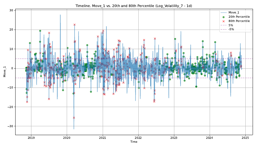
The large spikes visible from 2019 to 2021 are almost all marked red. The quieter 2023-2024 period shows a preponderance of green. The clustering is visible even without the t-tests.
The part that breaks it in live trading
The percentile thresholds are computed from the entire 2018-2024 dataset. P20 and P80 are fixed constants derived from the full history. That means from a 2019 vantage point those thresholds incorporate vol observations from 2020, 2021, 2022, and later years -- years that did not happen yet. This is not a minor efficiency issue; it is a structural look-ahead problem.
The paper acknowledges it directly in the Discussion section: "The primary limitation is the static nature of percentile calculation over time. Percentiles were derived from the entire dataset, which introduces periods where certain volatility states are under-represented or even absent. For instance, the year 2021 saw very few moves preceded by low volatility states." Look at the figure above: in 2021, log-vol spent almost its entire time above the 80th percentile band, because that band was calibrated on a dataset that includes the comparatively quiet 2023-2024 period. A trader running this in 2021 would see almost nothing classified as Low vol.
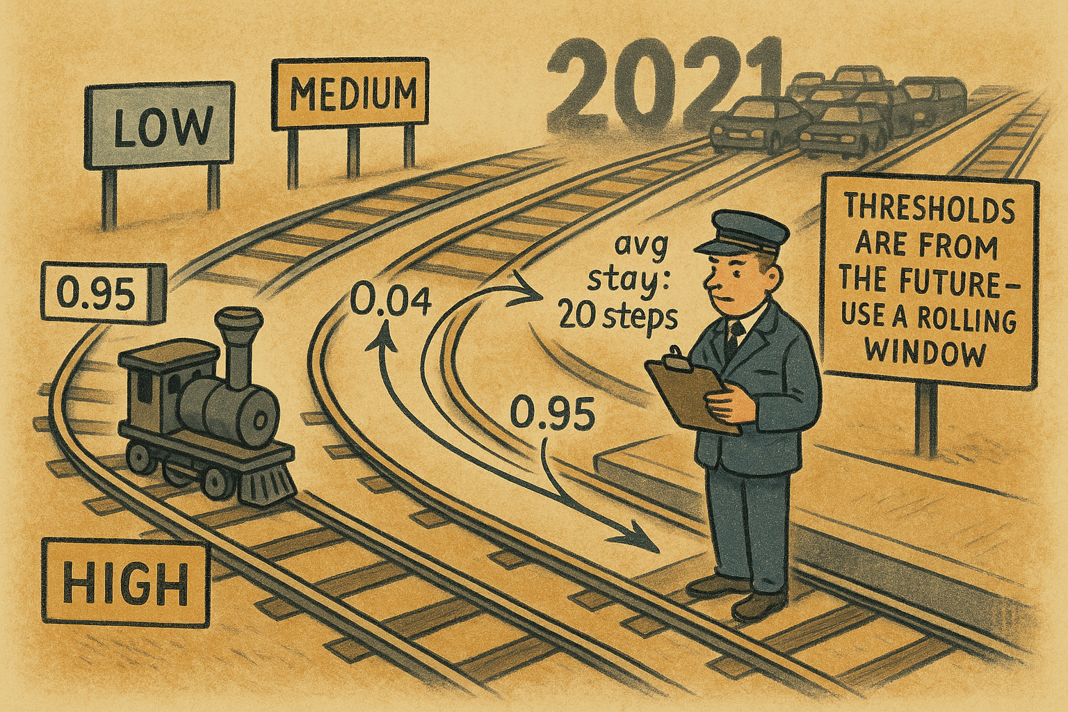
The fix the paper proposes is a rolling window for percentile computation: compute P20 and P80 using only the trailing year of data, then update the thresholds daily. That converts the static classification into an adaptive one. The paper does not implement this -- it is flagged as future work -- so the transition matrices and move statistics reported above are in-sample over the full period by construction. Treat them as an upper bound on what you would see in deployment.
The old article "Regime-Switching That Works, Factors That Don't (MS-GARCH)" covers a structurally similar problem from the other direction: MS-GARCH estimates regime parameters from the full sample, which creates similar in-sample favorability. The pattern repeats whenever regimes are defined post-hoc from aggregate statistics rather than estimated online.
The old article "Loose Pants Fit Everyone: Why General Trading Ideas Survive Longer" is relevant here too. A rule that says "expect quiet when vol is low" is loose enough to survive multiple market structures, even if the exact percentile thresholds shift. The direction of the relationship is durable; the magnitude in the tables above is not.
What the persistence does and does not tell you
A persistence of 0.95 in the High vol state does not mean vol will stay elevated for exactly 20 periods (1/0.05). It means each step has a 5% exit probability, giving a geometric distribution with mean 1/(1-0.95) = 20 periods, but the variance around that expectation is wide. You can be in High vol for 2 hours or 200 hours; the Markov model treats both as equally consistent with a 0.95 diagonal. What the matrix does give you is a prior for the next single step. If vol is High now, the probability that it exits to Medium in the next hourly bar is 3.7%, and the direct jump to Low is 0.03%. Building a hedge or sizing a position on that prior is sensible; sizing on "vol will stay High for the next 20 hours" is not.
The minimum persistence in the data (0.8167, 1d/7-period Low state) translates to a mean residence of 1/(1-0.8167) = 5.5 days. Short-window daily vol is visibly noisier, so the Low state exits more often. Once you switch to 90-day daily windows, the state is almost absorbing: mean residence at 0.9705 persistence is 1/(1-0.9705) = 34 days.
KEY POINTS
- Bitcoin log-volatility is stationary across all timeframes from 1h to 1d (except the 90-day daily window before differencing) and its ACF decays to near zero at lags beyond the computation window -- confirming persistence, not indefinite memory.
- A 3-state Markov chain (Low/Medium/High, split at the 20th and 80th percentile of log-vol) shows diagonal persistence above 0.9 in all but two cases across the entire study. The minimum is 0.8167 for the 1d/7-period Low state.
- In the High state, the 48-hour expected absolute move is 4.42% with a standard deviation of 4.37%, giving a mean-plus-one-sigma bound of roughly 9%. In the Low state, the 7-day expected absolute move averages 2.56% with std 2.81%; one-sigma boundary is 5.37%, not the "less than 5%" the paper text claims.
- The t-test between Low and High states rejects at t = -40.5 (1h data), confirming the difference is real. The Levene test confirms the variance gap too -- high state spreads are roughly 50% wider than low state spreads.
- The percentile thresholds are fixed on the full 2018-2024 dataset. This is a structural look-ahead: the P20/P80 values you see in the tables include post-sample data from the perspective of any date before 2024. A deployable version needs rolling-window thresholds.
- The framework works as a prior for option sizing and hedging, not as a point forecast. Persistence of 0.95 gives a mean residence of 20 periods, but variance around that is wide. Use the next-step transition probabilities, not the mean duration.
References
- Gyamerah (2019) — Modelling the Volatility of Bitcoin Returns Using GARCH Models — Quantitative Finance and Economics
- Yildirim & Bekun (2023) — Predicting Volatility of Bitcoin Returns with ARCH, GARCH and EGARCH — Future Business Journal
- Borrego Roldán (2024) — Volatility Clustering in Bitcoin — SSRN
A note on AI. The ideas, research, analysis, and conclusions in this article are my own. I use AI tools to help with editing and wordsmithing, because English is not my first language, and I am not shy about that. AI-generated ideas and AI-assisted writing are not the same thing: the first is empty slop from a generic prompt, the second is a tool for communicating years of real research more clearly. Judge the work by its substance, not by whether software helped polish the prose.