3.44 Quantitative Methods of Statistical Arbitrage: The Purdue Thesis Tour
Equity pairs: weight each spread by reversion speed over volatility times its OU fit. That book's daily Sharpe is 0.15 against 0.09 equal-weighted.

Ning's equal-weight book of six sector pairs earns a daily Sharpe of 0.09 in 2022. Daily Sharpe here is the mean daily percent return divided by the daily percent standard deviation, with no square root of 252 attached. You enter long when a pair's spread falls half a standard deviation through its 63-day average, and short when the spread rises the same distance above that average; you flatten when the spread crosses back through the average. Move that capital, once a quarter, toward the spreads that revert fastest per unit of noise, and the daily Sharpe on the book is 0.15. The weight is the product of two scores, each stretched from zero to one across the six pairs: the likelihood of a mean-reverting Gaussian fit, and the fitted reversion speed divided by the fitted volatility. In the fourth quarter that product leaves 0.78 of the book in Waste Management versus Republic Services.
The hedge is the ratio that makes the spread look like an OU
The six pairs are hand-picked sector twins: Waste Management with Republic Services, United with Delta, Visa with Mastercard, Morgan Stanley with Goldman Sachs, Nvidia with AMD, and Chevron with Exxon Mobil. Formation is calendar 2021. Trading is calendar 2022. Prices are Yahoo adjusted closes. The old article "Stat-Arb Is a Clustering Problem: Multi-View Spectral > Any Signal" finds that the grouping of names moves the result more than the signal you hang on the group. Ning never runs that comparison. He writes down the pairs a chart-watcher would have written down.
The spread at the hedge ratio B is the first leg minus B times the second.
$$ X_t = S_t^{1} - B\, S_t^{2} $$
B is the number you search. Ning grids it from -2 to 2 in steps of 0.01 and keeps the value that makes the historical spread look most like an Ornstein-Uhlenbeck process, a Gaussian pulled toward a long-run mean θ at speed μ with diffusion scale σ. On 2021 data the Waste Management hedge lands at 0.98 with an average log-likelihood of 5.71. Nvidia versus AMD lands at 1.31 with a score of 2.84, the worst fit of the six. Visa versus Mastercard is the best fit, at 0.99 and 5.83.
Given a candidate hedge, each day's spread is one Gaussian transition. The conditional mean is the previous spread decayed by e to the minus μ Δt, plus the long-run mean times whatever decay has not happened yet. The conditional variance is the usual OU one-step variance.
$$ m_i = x_{i-1} e^{-\mu \Delta t} + \theta \bigl(1 - e^{-\mu \Delta t}\bigr), \qquad \tilde\sigma^{2} = \sigma^{2} \frac{1 - e^{-2\mu \Delta t}}{2\mu} $$ $$ \log f(x_i \mid x_{i-1}) = -\tfrac{1}{2}\ln(2\pi) - \ln(\tilde\sigma) - \frac{(x_i - m_i)^{2}}{2\tilde\sigma^{2}} $$
The score he maximizes is the average of those log densities over the formation window. One step, using the 2022 Waste Management estimates and a one-day time step: μ is 0.1415, θ is 0, σ is 0.0193, the previous spread is 0.10, and the next spread is 0.08. The conditional mean is 0.10 times e to the -0.1415, which is 0.0868. The conditional standard deviation is 0.0180. The residual is -0.0068. That one observation contributes a log density of 3.03. His printed scores, between 2.93 and 5.89 on the 2022 fits, are averages of contributions on that scale. A tighter residual, or a smaller conditional standard deviation, pushes the average up through the minus-ln term.
He also prints a closed form for θ, μ, and σ. The expression for θ matches the usual regression of the spread on its lag: on a noise-free autoregression with true mean 2, his formula returns 2. The sum he labels X_yy is defined as the sum of lagged squares, the same sum he already labeled X_xx. The closed form for σ uses that sum, so I left the printed volatility expression unused. Fit the transition above on the grid of B. Do not implement the broken sum.
The trade on X is a band around an M-day moving average. In the backtest M is 63 and the half-deviation book uses K = 0.5. He also runs 0.75, 1, and 1.25.
$$ \begin{aligned} \text{long if } & X_t < MA - K \cdot SD, \\ \text{short if } & X_t > MA + K \cdot SD, \\ \text{flatten a long if } & X_t > MA, \\ \text{flatten a short if } & X_t < MA. \end{aligned} $$
MA and SD are the mean and standard deviation of the past M spreads. Worked band: the average is 100 and the standard deviation is 2, so K = 0.5 puts the long trigger at 99 and the short trigger at 101. A spread at 98.7 is a long. It comes off when the spread crosses back above 100. He defines a stop at a fixed fraction through the entry price and then says the experiments do not use it.
Speed over volatility, times the fit, and the worst pair gets zero
Ning calls the allocation mean reversion budgeting, MRB. Two indexes, both min-maxed across the pairs so the worst pair scores 0 and the best scores 1. The first is the maximized average log-likelihood. The second is the reversion speed divided by the diffusion scale.
$$ \hat\mu_i^{r} = \frac{\hat\mu_i}{\hat\sigma_i}, \qquad \bar\mu_i = \frac{\hat\mu_i^{r} - \min_j \hat\mu_j^{r}}{\max_j \hat\mu_j^{r} - \min_j \hat\mu_j^{r}}, \qquad \tilde\ell_i = \frac{\hat\ell_i - \min_j \hat\ell_j}{\max_j \hat\ell_j - \min_j \hat\ell_j} $$ $$ w_i = \frac{\bar\mu_i \, \tilde\ell_i}{\sum_{j=1}^{N} \bar\mu_j \, \tilde\ell_j} $$
Min-max on a single number is undefined; the minimum and the maximum run across the N pairs. The product in the numerator is why a pair dies twice: once for being the slowest, once for being the worst fit. Either zero kills the weight.
He prints μ, σ, and the likelihood for the full year 2022, and he prints quarterly weights. Those are different calculations. The quarterly inputs are not in the dissertation, so the full-year table cannot rebuild the backtest weights. It can show what the formula does. If the likelihood's time step is one day, the half-life ln(2)/μ is 4.90 days for Waste Management, 0.95 days for United-Delta, 64.2 days for Visa-Mastercard, 0.25 days for Nvidia-AMD, and 0.30 days for Chevron-Exxon. He never states the time unit. The ranking of μ/σ is what enters the weight, and that ranking is shared by every pair estimated on the same grid.
| Pair | μ | σ | likelihood | μ/σ | weight |
|---|---|---|---|---|---|
| WM-RSG | 0.1415 | 0.0193 | 5.7888 | 7.332 | 0.249 |
| UAL-DAL | 0.7284 | 0.0316 | 5.2948 | 23.051 | 0.688 |
| V-MA | 0.0108 | 0.0175 | 5.8850 | 0.617 | 0.000 |
| MS-GS | 0.0357 | 0.0244 | 5.5570 | 1.463 | 0.029 |
| NVDA-AMD | 2.7227 | 0.2594 | 3.1927 | 10.496 | 0.034 |
| CVX-XOM | 2.3461 | 0.3394 | 2.9276 | 6.912 | 0.000 |
Visa has the best likelihood, 5.8850, and the smallest speed ratio, 0.617. Its normalized speed is 0, so its weight is 0. United-Delta has the largest speed ratio, 23.051, so its normalized speed is 1. Its likelihood normalizes to (5.2948 − 2.9276) / (5.8850 − 2.9276) = 0.800. The product is 0.800. Chevron's likelihood is the minimum, so its normalized fit is 0 and its product is 0 even though the half-life, on a one-day step, is 0.30 days. Sum the six products and you get 1.163. United-Delta's weight is 0.800 / 1.163 = 0.688. Speed without a fit, and a fit without speed, both receive nothing. One fast, decently fitting pair takes about two thirds of this particular estimate.
The backtest weights, which you cannot rebuild from that table, concentrate harder and on a different name.
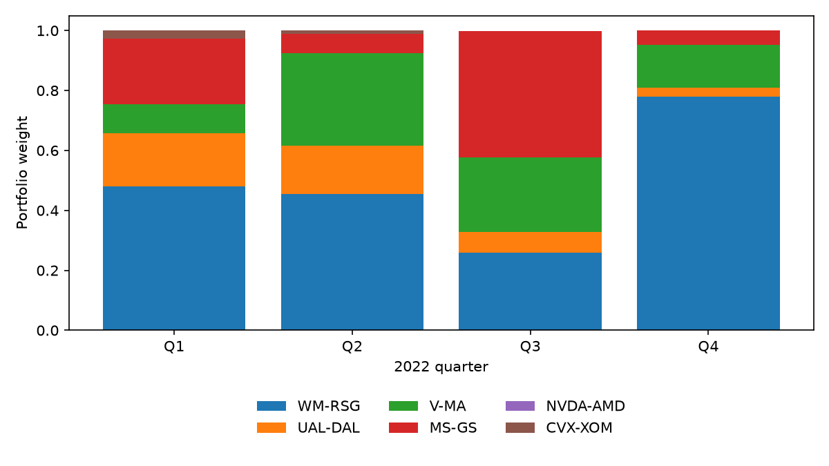
Look at the blue block in the fourth quarter. Waste Management versus Republic Services carries 0.78. Nvidia versus AMD is 0.00 in all four quarters. Chevron versus Exxon is 0.027, then 0.010, then 0. The first quarter still has five names with a nonzero weight. By the fourth quarter two names are alive in any size, and one of them is the book. Equal weight was the diversification. MRB is a tilt that is allowed to become a single pair.
The daily Sharpe on the half-deviation MRB book is 0.0410 / 0.2755 = 0.1488, which is the 0.15 in the opening, against 0.0260 / 0.3020 = 0.0861 for equal weight. Multiply 0.1488 by the square root of 252 and the ratio annualizes to 2.36. That 2.36 is one year, six names, and a commission of zero. The annual profit and loss printed next to the MRB Sharpe is 10.73%. Multiply 0.0410% by 252 and you get 10.33%. Compound that daily mean over 252 days and you get 10.88%. He does not say which aggregator produced 10.73%. The equal-weight row has the same unset total: 0.0260% a day and 6.62% on the year, while 252 times 0.0260% is 6.55%. I am leaving both annual figures as printed. The ratio that divides cleanly is the daily Sharpe.
Equal weight cuts volatility. At the half-deviation band the single-pair daily standard deviations run from 0.46% to 1.08%, and the book's is 0.30%. Ning reports the most positive correlation among the six spreads at about 0.3, which is the mechanical reason. At that band the best single pair still leads the book on Sharpe: Waste Management versus Republic Services alone prints 0.10, against the book's 0.09.
He also ranks the pairs, because the product can put most of the book in one name. Mean reversion ranking, MRR, sorts pairs by the same two ingredients and pays a fixed ladder. Start from equal weight 1/n, cut the worst pair in half, and hand the saved half to the best pair. The middle ranks step up evenly. For n pairs, worst to best:
$$ \left( \frac{n-1}{2n(n-1)},\; \frac{n+1}{2n(n-1)},\; \ldots,\; \frac{3(n-1)}{2n(n-1)} \right) $$
For six pairs the denominator is 60 and the numerators are 5, 7, 9, 11, 13, 15. The weights are 0.083, 0.117, 0.150, 0.183, 0.217, and 0.250. They sum to 1. The worst pair keeps a twelfth of the book, and the best pair gets a quarter.
The third allocator maximizes last quarter's Sharpe, and the objective is printed without the square root.
$$ w^{\ast} = \arg\max_{w} \frac{w^{\top} R}{w^{\top} \Sigma w} \quad \text{subject to} \quad \|w\|_{1} = 1 $$
R is the vector of average pair returns and Σ is their covariance. A Sharpe ratio divides by the square root of w-transpose Σ w. The printed ratio divides by the variance. Worked units: let w-transpose R equal 0.04 and w-transpose Σ w equal 0.16. The printed score is 0.25, in units of one over return. The Sharpe ratio is 0.04 / 0.40 = 0.10, dimensionless. He also writes ω on the left-hand side and w inside the objective. Leave the printed ratio as a warning. The book he labels mean-variance analysis finishes last at every band he tries. Chasing last quarter's return, on six pairs and one year, loses to equal weight.
The entry arrives when a signature score fills past 0.05
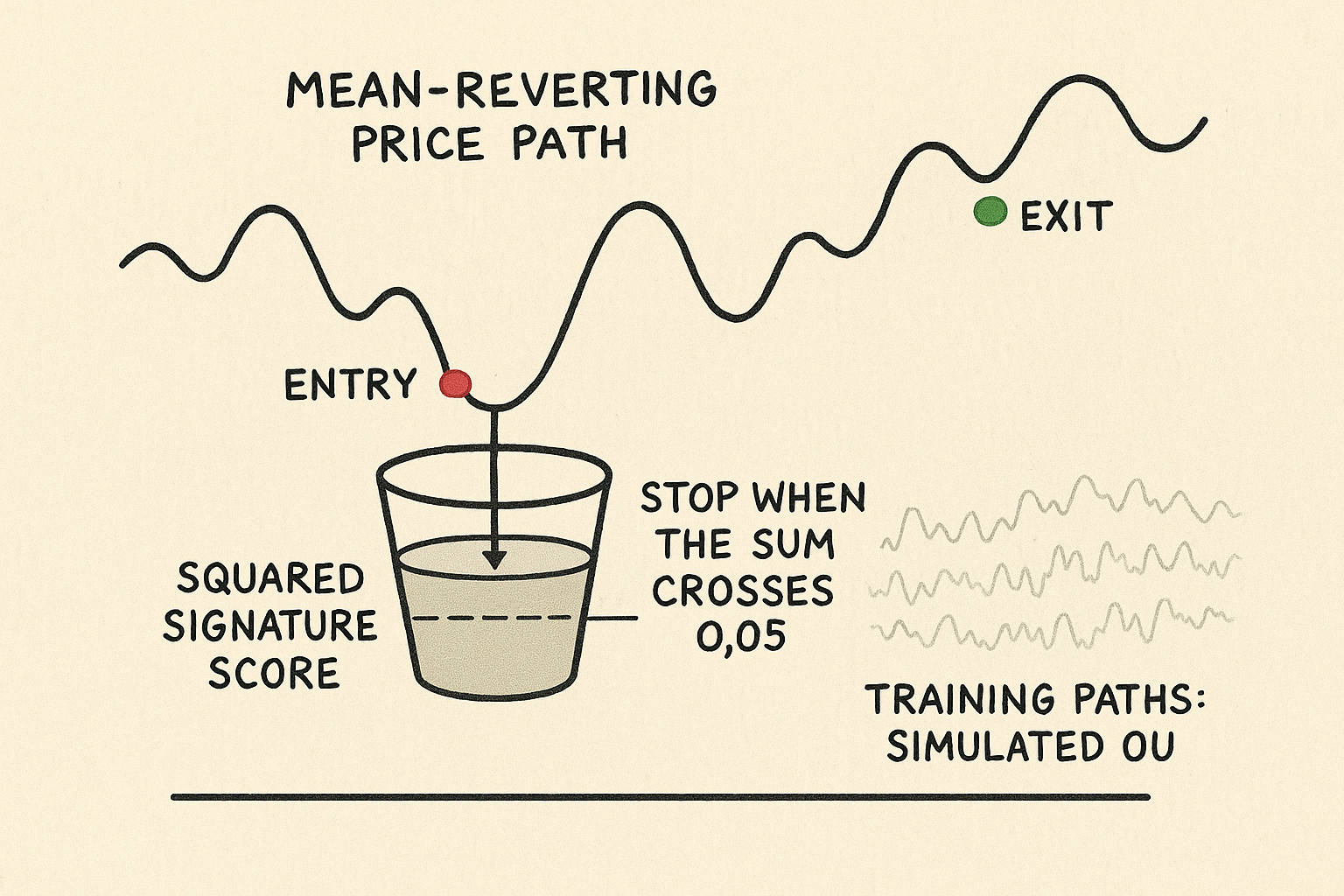
The second chapter of the dissertation times the entry and the exit. A signature of a path is the collection of its iterated integrals: the net move, then the integrals of moves against earlier moves, up to a truncation order. Ning time-augments the spread, so the path he transforms is the clock paired with X. A linear function of that truncated signature is the score. You stop at the first index where the running sum of squared scores crosses a constant k.
$$ \nu = \inf\left\{ j \ge 0 : \sum_{i=0}^{j} \langle \ell,\, \widehat{\mathbb{X}}_{0, t_i}^{\le N} \rangle^{2} \ge k \right\} $$
The stock test sets k to 0.05. He does not print the truncation order N, and he does not print the fitted linear coefficients. Worked arithmetic of the stopping rule, with a squared score of 0.01 chosen so the sum is easy to see: the running total is 0.01, 0.02, 0.03, 0.04, 0.05. You stop at j = 4. Without the scale of the linear function, 0.05 is a number you cannot transfer to another spread.
The long entry maximizes a discounted payoff that wants the spread to be low, net of a cost c.
$$ Y_t = e^{-r t} \bigl(-X_t - c\bigr) $$
You buy the low print. With r at 0 and c at 0.05, a spread of 98 scores Y = -98.05 and a spread of 102 scores Y = -102.05. The optimizer prefers 98. The exit leg flips the sign and subtracts an exit cost, so you sell the high print. He solves entry, then exit, then entry again, each time resimulating paths that start at the spread value where the previous stop landed. The equity writeup never gives a number for r or for c. If you put r at 5% a year anyway, a 20-day wait multiplies the objective by e to the -0.05 times 20/252, which is 0.996. The discount is a small shove. The cost would be the real penalty, and the cost is the number he left out.
The training loss replaces a step function at k with a sigmoid, because a hard threshold has no gradient. He sets the sigmoid slope at 20. The OU speed is a different quantity, and the dissertation uses one letter for both.
$$ \hat F(x) = \frac{1}{1 + e^{-20(x - k)}}, \qquad \hat G(x) = 1 - \hat F(x) $$
At the threshold, x = 0.05, the sigmoid is 0.5. At x = 0, it is 0.269, so G is 0.731. At x = 0.15, it is 0.881, so G is 0.119. The loss is the negative of the average payoff, and G weights the payoff increment at each step. One step of that: G of 0.731 times a payoff increase of 0.2 contributes 0.146 to the path score you are maximizing. He minimizes the negative of that score to move the linear coefficients.
On simulated paths whose long-run mean is 10, the average level at the signature stop is 10.23, and he says the path maxima cluster near 10.4. That is a small lift over stopping at the mean. The stopping level moves with volatility: 10.00 at σ = 0.1 and 10.52 at σ = 2, with the speed held at the setting he labels 10. Chapter 2 writes the OU with μ as the speed and θ as the mean. The simulation section swaps those two letters in the differential and still treats 10 as the long-run mean. I kept chapter 2's letters. The table's behavior, a stopping level stuck near 10 while the first column runs from 1 to 20, agrees with that reading.
The equity test is four of the same pairs, formed in 2021 and traded in 2022. He calls the framework free of assumptions on the spread. The training paths in this test are simulated from an OU fit. The baseline he beats is a different band from the allocation chapter: enter at 0.1 standard deviations and compute the mean and the standard deviation on 100 days. Chapter 2's loosest band is 0.5 on 63 days.
Count the days from an extreme back to the mean
The third chapter picks the hedge without an OU likelihood. Empirical mean reversion time, EMRT, is the average number of steps from an important extreme back to the sample mean. An important minimum is a point that is the low of some window, with both endpoints at least C sample standard deviations above it. An important maximum is the same idea upside down. In the simulation C is 2.
$$ X_m = \min_{i \le u \le j} X_u, \qquad X_i - X_m \ge C s, \qquad X_j - X_m \ge C s $$
Worked window, with s = 1 and C = 2, so the bar is 2. The values from index 0 through 6 are 3.0, 1.0, 0.2, -0.4, 0.5, 1.1, 2.5. The minimum is -0.4. The left endpoint clears it by 3.4 and the right endpoint clears it by 2.9. Both clear 2, so -0.4 is an important minimum. A shallow dip whose endpoints sit only 0.4 above it fails the same test.
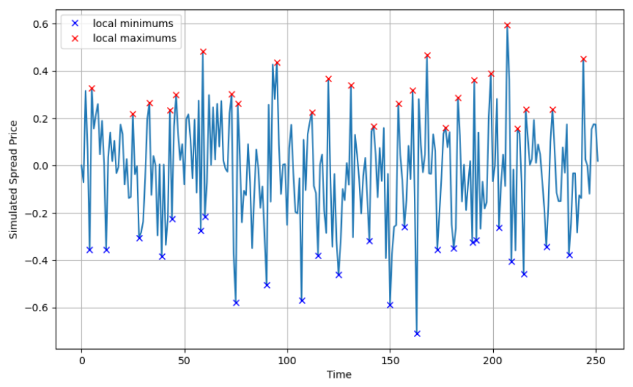
The red marks and the blue marks are the starts of the clock. The clock stops at the next crossing of the sample mean, which this figure does not label. Odd timestamps in the prose are extremes of either sign. The displayed formula for the odd timestamps says "local maximum" only. I followed the prose, minimum or maximum, and I am flagging the formula line.
$$ r = \frac{2}{N} \sum_{\substack{n=2 \\ n \text{ even}}}^{N} (\tau_n - \tau_{n-1}) $$
N is the number of timestamps. The sum keeps the even gaps only, extreme to mean, and drops the time spent traveling back out to the next extreme. The factor 2/N turns that sum into an average when half the timestamps are crossings. His source line mixes the index i with the index n; the expression above is the same average with one index. Worked timestamps: an extreme at 5, a crossing at 12, an extreme at 20, a crossing at 28. The even gaps are 7 and 8. With N = 4, r = (2/4) times (7 + 8) = 7.5. Four timestamps, two reversion legs, average length 7.5.
On simulated OU paths of 1,000 points, that average falls as the speed rises: 98.79 steps at speed 2, and 31.15 steps at speed 20, with C = 2. The direction is what you want from a reversion clock. He then sets the first coefficient to 1 and grid-searches the others to minimize r. The grid line as printed jumps from -2.99 to -0.98. I left that gap as printed. The coefficient table is still usable, and one entry matters.
CVS versus Johnson & Johnson gets an EMRT coefficient of -0.24. The spread is the first price minus B times the second, so a negative B is long both names. Distance-method B on that pair is 1. The OU likelihood B is 0.43. Minimizing time-to-mean turned a pair into a same-direction book. The coefficient table also prints MSFT-GOOG where the performance table prints MSFT-GOOGL, and CL-KMIB where the other tables print CL-KMB. I used the performance-table tickers.
The reward uses a mean the market will not hand you
The same chapter then trades the spread with tabular Q-learning. The state is the last l daily percent moves, each crushed into four bins. He sets l to 4 in the simulation and says that produces 16 states. Four bins to the fourth power is 256. I am keeping his sentence and flagging the count.
$$ \pi_i = 100 \cdot \frac{P_i - P_{i-1}}{P_{i-1}}, \qquad d_i = \begin{cases} +2 & \pi_i > k \\ +1 & 0 < \pi_i < k \\ -1 & -k < \pi_i < 0 \\ -2 & \pi_i < -k \end{cases} $$
With k at 3, a move from 100 to 103.5 is +3.5%, which bins as +2. A move from 100 to 101.5 is +1.5%, which bins as +1. A move from 100 to 96 is -4%, which bins as -2. A flat day, and a move of exactly k percent, match none of the four cases as printed. From a flat position the allowed actions are buy one share or do nothing. From a long, the allowed actions are sell one share or do nothing.
The reward pays the action for the distance to the mean, minus a cost on the trade.
$$ R = A \, (\theta - X) - c \, |A| $$
θ is the mean of the spread and A is the share action, +1, 0, or -1. Worked buy: θ is 100, X is 97, c is 0.1, A is +1. The reward is 3 − 0.1 = 2.9. The same cost on a sale at 103 is −1 times (100 − 103) minus 0.1, which is also 2.9. Add the two rewards and θ cancels: 5.8, equal to the price change of 6 minus two costs of 0.1. On a completed round trip the sum of the rewards is the spread profit and loss. The mean only decides which leg is credited. A wrong mean still totals to the profit and loss, and it assigns the credit to the wrong state. The state you act on is the recent-return bins. θ sits in the reward. He trains on simulated OU paths, where that mean is the one he typed in, then deploys the table on stocks. By decision time the mean is already inside the table. Building the table is where you needed it, to decide which simulated states were worth buying.
He writes a second objective that adds the terminal inventory times the raw spread level. A reward of 2.9 next to a terminal add-on of about 100, if you finish long one share of a spread near 100, is a different scale. The training OU is centered at 1, where the same add-on is about 1 against rewards of a tenth, and it still dominates a single reward. The update he says he runs is ordinary Q-learning, so that is the iteration to implement.
$$ Q \leftarrow Q + \alpha \left( R + \gamma \max_{a} Q_{\text{next}} - Q \right) $$
Worked step, with his simulation settings α = 0.1 and γ = 0.99. Start at Q = 1, earn R = 2.9, and let the best next action be worth 1.5. The target is 2.9 + 0.99 times 1.5 = 4.385. The new Q is 1 + 0.1 times (4.385 − 1) = 1.3385. Exploration during training is 0.1; at test time it is 0. He runs 10 episodes. The implementation still chooses the bin width, the lookback of 4, the learning rate, the discount, the exploration rate, and the episode count. The distance-method benchmark enters at one sample standard deviation. The OU benchmark enters at 0.5 equilibrium standard deviations.
$$ \hat\sigma_{\mathrm{eq}} = \frac{\hat\sigma}{\sqrt{2\hat\mu}} $$
That equilibrium scale is the stationary standard deviation of the OU. Chapter 2's band uses a 63-day standard deviation. Using the 2022 Waste Management estimates, because the trading chapter does not print μ and σ for its ten pairs: 0.0193 / sqrt(2 times 0.1415) = 0.0363. Half of that is the OU entry distance under his k = 0.5. A reader who lines this band up with chapter 2's K = 0.5 is lining up two different rulers.
The evaluation on simulated paths deploys all cash at each buy. The action definition is one share. The writeup reports an average profit above 600% on 100 fresh OU paths from a 100 dollar start. That number lives on the process the reward was written for, with the simulated mean inside the credit. I am not carrying it to a stock account.
Look at the orange line in the loose-band panel

Look at the orange line in panel (a), the half-deviation band. It finishes near the printed MRB profit, above equal weight and above the red mean-variance line, which gives back a chunk of the year around the middle of the sample and never catches up.
At that band the daily Sharpes are 0.15 for mean-reversion budgeting, 0.09 for equal weight, and 0.06 for the mean-variance book. At a one-standard-deviation band those four daily Sharpes are 0.18, 0.17, 0.19, and 0.06; the signature rule, against a 0.1-standard-deviation baseline, lifts United versus Delta from a daily Sharpe of 0.05 and a 9.64% year to 0.18 and 42.46%, while Goldman versus Morgan Stanley draws down 7.90% against 2.25% on that same baseline; the ten reinforcement-learning daily Sharpes in 2023 run from 0.05 to 0.14.
One year, no commission, and a 0.78 weight
I am against putting capital on this dissertation. The piece worth keeping is the tilt: among spreads you already trust, give more weight to a high speed-over-volatility ratio and a high OU likelihood, and refuse the min-max that zeroes names and can hand one pair 0.78. The ranking ladder, a twelfth on the worst name and a quarter on the best, is the version that still diversifies. Recompute the weight every quarter from that quarter's own μ, σ, and likelihood. Ning's full-year parameter table is a different fit from those quarterly inputs.
The old article "Building a Trend Follower, Component by Component" treats commission as a component of the system. Ning writes a cost into the signature payoff and into the Q-learning reward, and the equity tables contain no value for it. Chapter 2 writes a stop and turns it off. Each test is one year: 2022 for the allocation and the signature, 2023 for the reinforcement learner, after a prior year of formation, with the commission left at zero. The flattering allocation gap is the loosest of four bands. Tighten the band to one standard deviation and MRB's daily Sharpe, 0.18, sits a hundredth above equal weight, and the ranking book is the one ahead.
Reproducing a signature entry takes the truncation order, the linear coefficients, and the cost. He prints none of the three. He does print that the training paths were drawn from an OU, and that the baseline band is 0.1 on a 100-day window. A 42% year on United versus Delta against that baseline is a research exhibit.
The reinforcement learner is long-only, trained where the mean is known, and scored on ten sector pairs he chose. Before you quote a cell, divide the printed daily return by the printed daily standard deviation. They match across the tables I checked, except OXY versus Exxon under the RL column: 0.0609 / 0.9446 = 0.064, and the printed daily Sharpe is 0.086. I am leaving 0.086 in place and treating that cell as a possible source error. The same pass is why the annual profit of 10.73% stays next to a daily mean that does not multiply out to it.
If you build the tilt, cap the weight, charge a commission you measured, and make the pair list earn its place against a dumb equal-weight book on a second year. The signature timer and the Q-learner stay in the lab until the cost is a number and the mean inside the reward is a mean you will have on the day you trade.
KEY POINTS
- Weight a multi-pair equity book by reversion speed over volatility times the OU likelihood. At a half-standard-deviation band that book has daily Sharpe 0.15 against 0.09 equal-weighted.
- Min-max both scores before you multiply. The slowest pair and the worst fit go to zero, and the fourth quarter of the backtest puts 0.78 in Waste Management versus Republic Services.
- Use the rank ladder when every name has to keep a weight. On six pairs the worst name keeps 1/12 of the book.
- Time an entry by accumulating a squared signature score until it crosses 0.05, and know the stock test fit that score on paths simulated from an OU.
- Check the EMRT hedge sign before you call it a pair. CVS versus Johnson & Johnson prints -0.24, long both legs.
References
- Stat-Arb Is a Clustering Problem: Multi-View Spectral > Any Signal
- Building a Trend Follower, Component by Component
- Quantitative Methods of Statistical Arbitrage, Boming Ning
A note on AI. The ideas, research, analysis, and conclusions in this article are my own. I use AI tools to help with editing and wordsmithing, because English is not my first language, and I am not shy about that. AI-generated ideas and AI-assisted writing are not the same thing: the first is empty slop from a generic prompt, the second is a tool for communicating years of real research more clearly. Judge the work by its substance, not by whether software helped polish the prose.