3.41 Stat-Arb Is a Clustering Problem: Multi-View Spectral > Any Signal
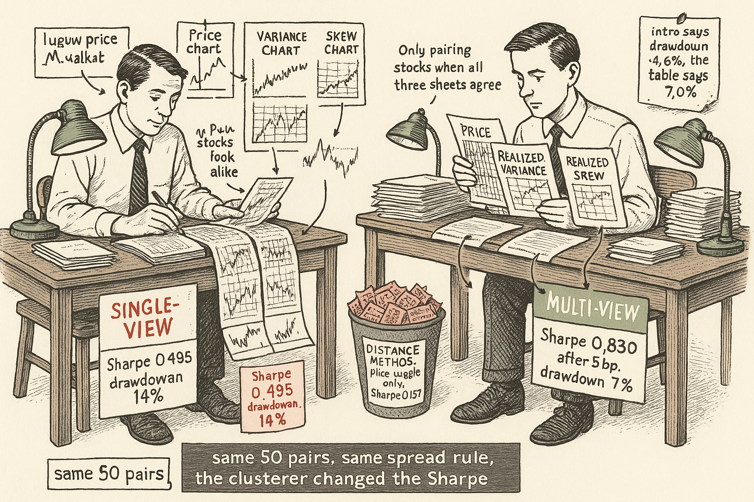
S&P 500 pairs, 2000-2022: multi-view spectral clustering posts Sharpe 0.830 after 5bp. Price-distance pairs fall to 0.338, and the paper's 4.6% drawdown is missing from its table.
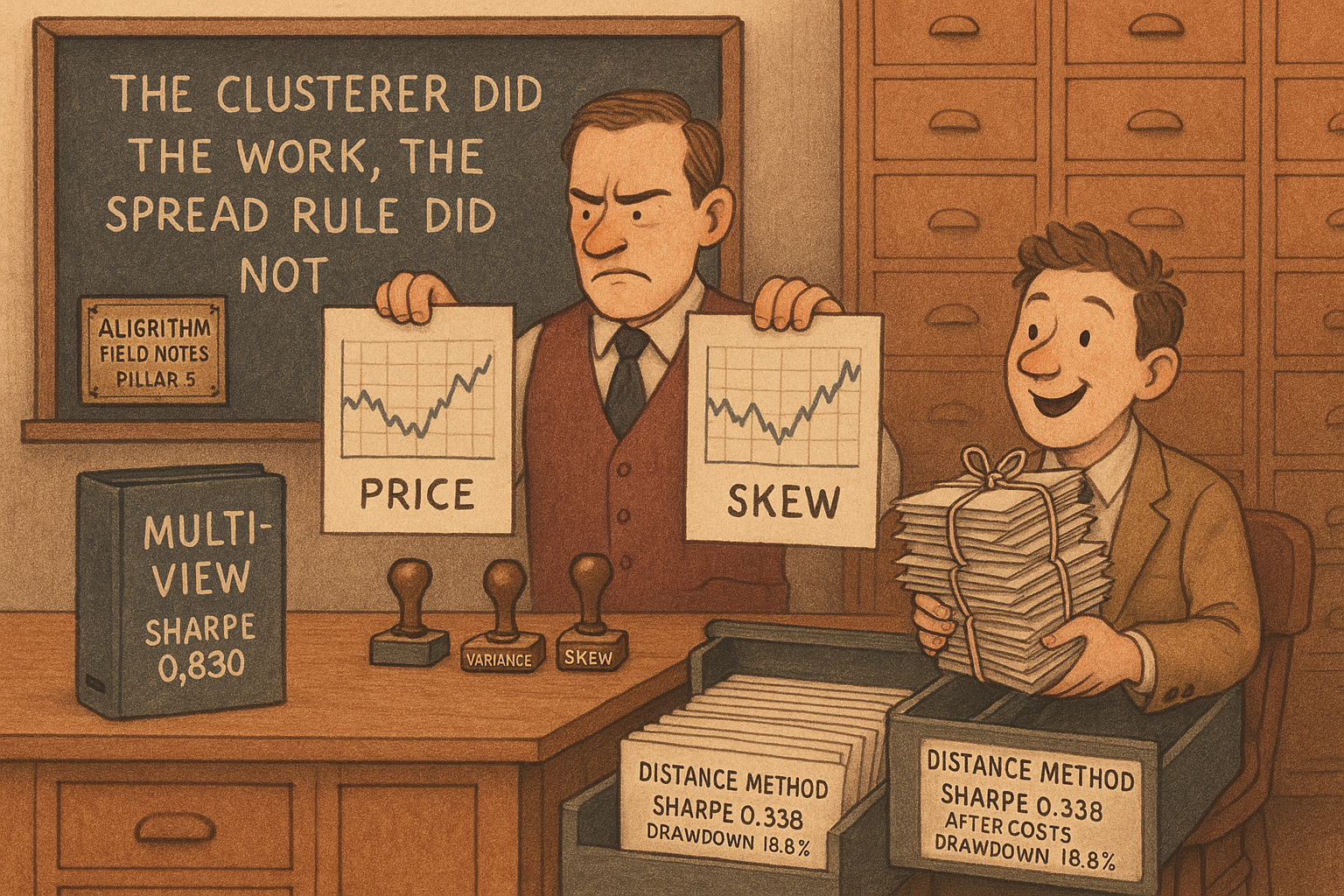
On S&P 500 names from 2000 to 2022, the best book in Raymond Leung's grid is multi-view co-regularized spectral clustering with 25 clusters, a plain long-short spread, and an Ornstein-Uhlenbeck entry and exit. After a 5 basis point charge on each leg at entry and again at exit, that book has an annualized Sharpe ratio of 0.830, a mean excess return of 2.7% a year, and a maximum drawdown of 7.0%. Hold the feature set fixed at the full intraday menu and the cost fixed, and the best distance-method book falls to a Sharpe ratio of 0.187. The best single-view book falls to 0.495. The clusterer moves the Sharpe ratio. Changing the signal inside one clusterer moves it less. The introduction also prints a pre-cost Sharpe ratio of 1.166 and a 4.6% drawdown for that same best book. No results table prints either figure. The after-cost table prints 7.0%.
What this actually is
You run pairs on the S&P 500. The formation window is 252 business days, the trading window is the next 126, and the book holds 50 pairs. The classical membership test asks whether two normalized price paths stayed close over the formation window. Leung's claim is that this test admits pairs whose one-minute variance, skew, and betas disagree, and those are the pairs whose gaps fail to close.
The method builds a separate similarity graph for each feature, the closing price included, fuses the graphs, and cuts the result into clusters before any spread rule runs.
Think of a stack of tracing sheets. One sheet is the price path. The next is realized variance. The next is realized skew. Single-view clustering glues the sheets into one long strip and measures distance along the strip. Multi-view clustering leaves each sheet intact, draws a who-resembles-whom map on each sheet, and keeps the pair when the maps agree. A price match that fails the variance sheet loses its ticket.
If that claim holds at the desk, the research budget goes to the clusterer and to a one-minute realized-moment pipeline, and the entry rule can stay a plain spread threshold. If the claim is the winner of more than 2,000 specifications on the same 22 years, the cost of believing it is a data build whose published Sharpe ratio was the maximum of a search the paper does not haircut.
Price distance, after five basis points
Price distance on large-cap US names after 2000 is the benchmark, and after 5 basis points it does not clear a t-statistic of 2.
The formation window is 12 times 21, so 252 business days. The trading window is 6 times 21, so 126 business days. Six such trading windows overlap, the same staggered construction Gatev, Goetzmann, and Rouwenhorst used. A normalized price is that day's close divided by the close on the first day of the formation window.
The distance method keeps the 50 pairs with the smallest gap. Leung prints the gap as follows.
$$ \mathrm{MSE}_{ij} = \frac{1}{T} \sum_{t=1}^{T} \| z_i - z_j \|_2^2 $$
Read it as: z_i is the stacked feature path of name i, a vector of length p times T, where p is the number of features and T is 252 formation days. The double-bar is Euclidean length. As printed, the quantity inside the sum does not depend on the day index t, because z_i already contains every day. The sum therefore collapses, and the whole expression equals the squared Euclidean distance between the two stacked paths. Dividing by T, or skipping that division, does not change which 50 pairs win. On price alone, that distance is the sum of squared gaps in the normalized price index, which is the Gatev ranking.
Worked on three formation days. Name A prints 1.00, 1.02, 1.01. Name B prints 1.00, 1.05, 0.98. Squared gaps are 0, 0.0009, and 0.0009. The sum is 0.0018. The mean is 0.0006. Either number ranks this pair the same way against every other pair.
On price alone, the two-standard-deviation rule has a Sharpe ratio of 0.571 before costs and 0.338 after, with a drawdown of 18.8% after costs. The after-cost mean excess return is 1.5% a year. Divide 0.015 by 0.338 and the annualized volatility is 4.4%. The t-statistic on that mean is 1.545. Rad, Low, and Faff document the same fade on a broader CRSP universe: distance-method mean excess returns peaked near 1.80% a month in the early 1970s, which is 21.6% a year, and fell to about 0.20% a month by the 2010s, which is 2.4% a year. Leung's pre-cost mean on this rule is 2.6% a year, in that neighborhood, on a more liquid universe. Do and Faff asked whether simple pairs trading still works. Avellaneda and Lee, and Krauss's survey, report the same decline. On S&P 500 names after 2000, with 5 basis points, the classical book does not pay.
Moments from the one-minute tape
The extra features are one-minute moments, computed once a day, and they are what the multi-view books cluster on.
Leung's prose defines realized variance as the sum of squared one-minute log returns. That is the estimator in Andersen, Bollerslev, Diebold, and Labys. Table 2 of the paper prints a different expression, the sum of squared changes in those returns.
$$ \mathrm{RV}_{t,i} = \sum_{m=1}^{M} R_{t_m,i}^{2}, \qquad R_{t_m,i} = \log P_{t_m,i} - \log P_{t_{m-1},i} $$
Read it as: on day t, for name i, take each one-minute log return R, square it, and add across the M minutes in the day. P is the one-minute price. The sum is that day's realized variance, in the units of a squared log return. Leung uses a one-minute grid throughout.
Worked on three minutes: log returns 0.001, minus 0.002, and 0.0015. Sum of squares is 0.000001 plus 0.000004 plus 0.00000225, which is 0.00000725. The Table 2 first-difference form on the same three numbers, squared changes of the returns rather than squared returns, equals 0.00002125. The prose definition is the one that matches the paper he cites. Table 2 does not match the prose. The source may have transcribed the cell wrong. There is no code in the paper, so which expression built the clusters is not recoverable from the text. The rest of this article treats realized variance as the sum of squared one-minute log returns, and treats the table cell as unreliable.
Realized skewness and kurtosis follow Amaya, Christoffersen, Jacobs, and Vasquez.
$$ \mathrm{Skew}_{t,i} = \frac{\sqrt{M} \sum_{m=1}^{M} R_{t_m,i}^{3}}{\left(\sum_{m=1}^{M} R_{t_m,i}^{2}\right)^{3/2}}, \qquad \mathrm{Kurt}_{t,i} = \frac{M \sum_{m=1}^{M} R_{t_m,i}^{4}}{\left(\sum_{m=1}^{M} R_{t_m,i}^{2}\right)^{2}} $$
Read it as: skewness is the third-moment sum, scaled by the square root of the minute count M, divided by the realized-variance term to the power 3/2. Kurtosis is M times the fourth-moment sum, divided by the square of the sum of squares. Both are pure numbers. A negative skewness means the down minutes were fatter than the up minutes that day.
Same three returns. The sum of cubes is 0.000000001 minus 0.000000008 plus 0.000000003375, which is minus 0.000000003625. Skewness comes out at minus 0.322. Kurtosis comes out at 1.26. Three minutes is a toy day, enough to see the arithmetic, not a market fact.
He also builds upside and downside semivariance, and an intraday beta of each name on SPY and on the sector ETFs: realized covariance with the reference, divided by the reference's realized variance. Daily market, size, value, and momentum betas, plus idiosyncratic volatility and total volatility, sit on the same menu, from a trailing regression of 252 days with a minimum of 126. He standardizes each feature across names, one day at a time, to zero mean and unit standard deviation, before any clustering. The kitchen-sink collection, his feature set 14, is the one the best book uses. He labels it All.
One graph per feature
Single-view clustering flattens every feature into one vector. Multi-view clustering keeps a graph per feature. That split is the whole method.
With p features, single-view stacks the p matrices, each of size T by N, into one matrix of height p times T. Each name is one long vector. A price match and a variance match are the same Euclidean inches. Multi-view leaves the p matrices separate and builds one similarity per feature. Leung's local scale uses the distance to the 7th nearest neighbor.
$$ w_{ij} = \exp\left( -\frac{\| x_i - x_j \|^2}{\sigma_i \, \sigma_j} \right) $$
Read it as: w_ij is the similarity of names i and j on one feature, a number between 0 and 1. x_i is that name's T-day path on the feature. Sigma_i is the distance from i to its 7th nearest neighbor on the same feature. Closer paths produce a larger weight.
Worked: squared distance 0.25, sigma_i equal to 1, sigma_j equal to 0.5. The fraction inside the exponent is 0.25 divided by 0.5, so 0.5. The weight is e to the power minus 0.5, which is 0.607.
From that similarity matrix W he builds the symmetric normalization D to the power minus one half, times W, times D to the power minus one half. D is the diagonal matrix of row sums. He takes the top K eigenvectors, rescales each row to length 1, and runs k-means. That is his single-view spectral step, the procedure of Ng, Jordan, and Weiss. K is either 10 or 25. He says he has no rule for the right K once several views are fused, so the two values are a sensitivity check. A single pairwise price gap is a thin graph, which is the complaint in the old article "Stop Using Pairwise Granger: PCMCI for Financial Causality". Multi-view clustering builds one similarity graph per feature and fuses them. It is a clustering step, not a search for causal parents.
The co-regularized multi-view step, his Algorithm 4, maximizes the sum across views of a trace term on each view's eigenvectors, plus a penalty, scaled by lambda, that rewards eigenvectors which agree across views. Each view's eigenvector matrix is constrained to have orthonormal columns. He freezes lambda at 1/2 and does not cross-validate it. He then runs k-means on the eigenvectors of the price view, which he treats as the most informative view. His reference list points this objective at Kumar and Daumé (2011). That paper's abstract says the method has no free parameter. The objective he prints has lambda. Keep his equation, and keep lambda at 1/2 as an untested choice. The citation may point at the wrong writeup of the same idea.
Clusters from this cut can hold more than two names. He screens back to 50 pairs on the price gap, taking the ceiling of 50 divided by K pairs from each cluster, then the 50 smallest gaps overall. For K equal to 25 that is 2 pairs from each cluster. For K equal to 10 it is 5. The screen stops the list from collapsing into the single tightest cluster. He also notes that insisting on 50 pairs, where the pairs literature often keeps 20, pulls in worse price fits, and he treats that as a downward bias on the results.
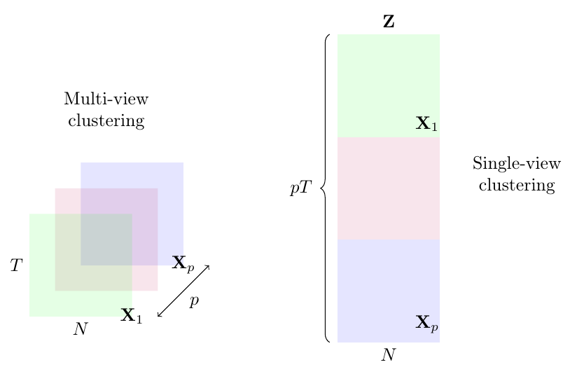
The left block is the multi-view input, one sheet per feature. The right block is the single-view input, the same sheets glued into one column. Everything after this picture is a consequence of which block you hand to the clusterer.
Fifty pairs, six months, five basis points
A cluster becomes a position through a spread, a threshold, and a 5 basis point toll on every leg at entry and at exit.
The plain signal is the undirected spread: normalized price of name 1 minus normalized price of name 2. The direction of the trade is fixed when the spread crosses a threshold, not when the pair is chosen. The cointegration signal follows the Engle and Granger two-step in the form Rad, Low, and Faff use. Over the formation window he regresses each normalized price on the other, keeps the regression with the smaller Augmented Dickey-Fuller statistic, and sets the spread equal to P1 minus beta-hat times P2. The Dickey-Fuller statistic picks a direction. He does not require it to pass as a test of cointegration. The copula signal fits marginal distributions and a copula on formation returns, builds a cumulative mispricing index for each leg, and opens when the two indices sit on opposite sides of plus or minus 0.5, one dollar against one dollar. Multivariate cointegration, a Johansen vector on every name in the cluster, produced the worst books in the grid. He drops it from the rest of the reported results. Every Sharpe ratio below is a two-name trade.
The two-standard-deviation rule opens when the spread crosses the 2.5 or 97.5 percent point of the distribution fitted on the formation window, and closes when the spread crosses zero. He fits several distributions and keeps the one with the lowest AIC; the Gaussian case is the classical Gatev threshold, with the round percentiles 0.025 and 0.975 in place of a strict two-sigma cut. The Ornstein-Uhlenbeck rule models the spread as a reverting diffusion.
$$ dX_t = -\alpha X_t \, dt + \eta \, dB_t $$
Read it as: X is the spread. Alpha is the reversion speed per day. Eta is the diffusion scale, in spread units per square root of a day. B is a standard Brownian motion. He estimates alpha and eta by maximum likelihood on the formation window.
Bertram's optimal barriers are symmetric: enter at a-star, exit at minus a-star. Leung's cost input to that calculation is
$$ c = 2 \times 0.0005 \times \| \beta \|_1 $$
Read it as: 0.0005 is 5 basis points. The leading 2 makes it a round trip. The L1 norm adds the absolute values of the position weights. For a one-dollar long and a one-dollar short, beta is the pair (1, minus 1), the L1 norm is 2, and c equals 0.002. That is 20 basis points on one dollar of long notional, paid across both legs and both sides.
He also prints a maximand for the optimal entry. It has the shape alpha times (2a plus kappa), divided by 2 pi times an error function of the square root of alpha over eta. Kappa is never defined. The denominator does not depend on the entry level a, so the printed expression has no interior maximum. The operational rule is still usable: fit alpha and eta on the formation spread, charge that c, enter at a-star, exit at minus a-star. The maximand as transcribed is not. The source may have dropped terms. This article does not replace them with a repaired formula.
Daily portfolio return is an employed-capital average, following Gatev and Do and Faff.
$$ R_s = \frac{1}{L_s} \sum_{l=1}^{L_s} \mathrm{PnL}_{s,l} $$
Read it as: L_s is the number of trades open on day s, counted across all six overlapping windows. PnL of trade l is the dollar mark-to-market on a one-dollar long leg and a one-dollar short leg. The day's portfolio figure is the average of those dollar PnLs. He calls the series an excess return because the pair is dollar-neutral at the open and the accounting charges no financing.
$$ \mathrm{SR} = \frac{\overline{R}}{\sigma} $$
Read it as: the annualized mean of that excess-return series, divided by its annualized standard deviation. He uses 252 business days wherever he annualizes. No separate risk-free rate appears in the tables.
Worked on his own prices, with the arithmetic corrected. Long one dollar of a name at 100 dollars, short one dollar of the other at 5 dollars. The share counts are 0.01 and minus 0.2. At the open the position value is zero, and the open cost is 0.0005 times (1 plus 1), so 0.0010 dollars. At the close the long name is at 150 and the short name is at 3.50, against prior marks of 145.75 and 4.25. That day's mark-to-market is 0.01 times 4.25, plus minus 0.2 times (3.50 minus 4.25), which is 0.0425 plus 0.15, so 0.1925 dollars. The exit cost is 0.0005 times (1.50 plus 0.70), so 0.0011 dollars. From the open prices to the close prices the gross profit is 0.01 times (150 minus 100), plus minus 0.2 times (3.50 minus 5), which is 0.50 plus 0.30, so 0.80 dollars. Round-trip cost is 0.0021 dollars. Net is 0.7979 dollars.
His writeup of this same trade prints a gross of 0.20 dollars and a net of 0.1989. The 0.20 subtracts the short leg's gain instead of adding it. The 0.1989 then subtracts the exit cost alone, not the 0.0021 round trip. Both steps disagree with the share counts he set above them, which do produce the 0.1925 closing-day mark he also prints. The corrected totals are 0.80 gross and 0.7979 net.
The 5 basis point rate is the median market-impact cost Frazzini, Israel, and Moskowitz report for US equities, 5.08 basis points on NYSE-AMEX and 5.03 on NASDAQ, over 1998 to 2016. It is a large-cap number. He applies the same 5 basis points to ETFs, futures, and foreign exchange, and he says the cost literature off equities is thin. That flat rate on the other asset classes is his assumption.
The clusterer, then the signal
With the feature set held at All and costs turned on, the clusterer ranks the books, and the signal does not reorder that ranking.
The best distance-method row has a Sharpe ratio of 0.187 and a drawdown of 14.3%. The best single-view row has 0.495 and a drawdown of 14.0%. The best multi-view row has 0.830 and a drawdown of 7.0%. That row is co-regularized spectral clustering, K equal to 25, the All feature set, the bivariate long-short, and Ornstein-Uhlenbeck barriers. Its mean excess return is 2.7% a year and the t-statistic is 3.797. Divide 0.027 by 0.830 and the annualized volatility is 3.25%. Divide the t-statistic by the Sharpe ratio and square the result: 3.797 divided by 0.830, squared, is 20.9 years. That matches a 2000 to 2022 sample after a one-year formation. The distance-method rows produce the same 20.9 years. The mean, the Sharpe ratio, and the t-statistic are one identity.
The tenth-best multi-view row on that same All set still prints a Sharpe ratio of 0.611, above the best single-view row. Across feature subsets, the top of the after-cost table is a run of multi-view long-short Ornstein-Uhlenbeck books from 0.748 to 0.830. A copula row and a cointegration row sit inside the multi-view top ten, so no one signal owns the list. He reports the same for trading rules, in the supplement. The ordering that survives is distance, then single-view, then multi-view. Picking the 50 pairs is itself a ranking, and the old article "Ranking Beats Forecasting for Many Trading Problems" is the same moral in another setting: the ordering imposed on the names does more work than the forecast attached afterward. Here the ordering is the cluster assignment.
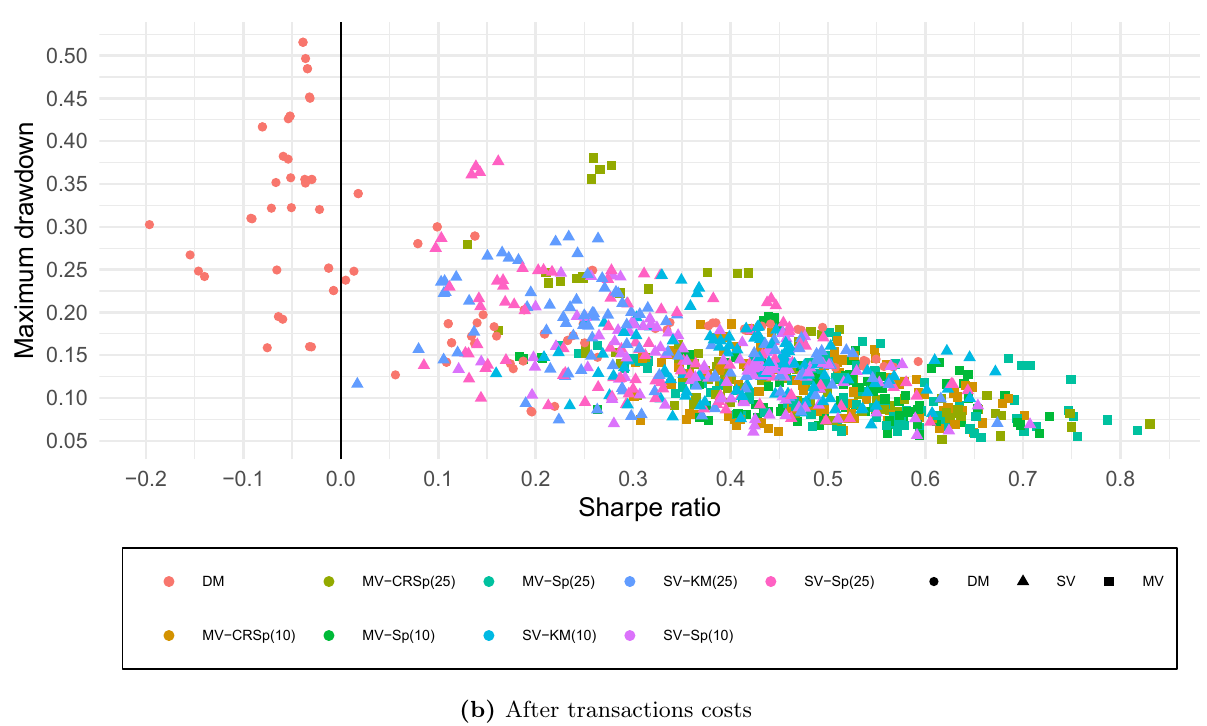
Red points are the distance method. Green and olive points are multi-view. The right edge of the cloud, Sharpe ratios out near 0.8 and drawdowns near 7%, is multi-view. A mass of red points sits left of zero, with drawdowns from about 15% to about 50%. He says the grid contains well over 2,000 combinations, and he cites Harvey, Liu, and Zhu on multiple testing. His answer is the top-down sort and the plateau: many multi-view rows land near one another. He does not report a deflated Sharpe ratio. The plateau is in the table. The 0.830 is still the maximum of a search over one 22-year path.
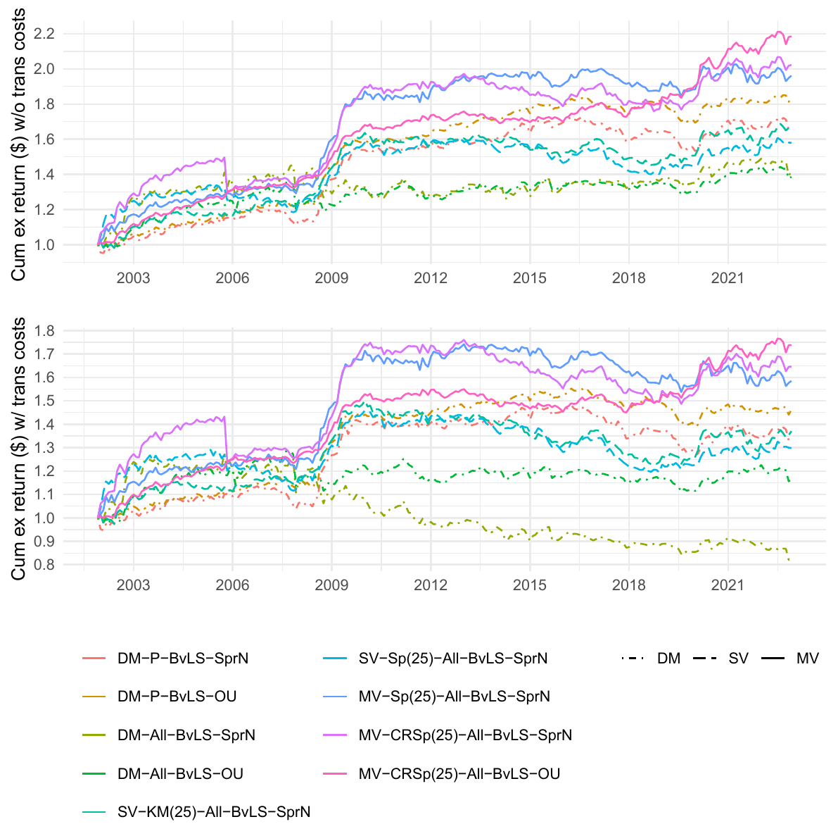
The lower panel is after costs. The pink line is the best book and finishes near 1.75 dollars per starting dollar. The olive dash-dot line is the distance method on the same All feature set with the two-standard-deviation rule, and it finishes near 0.85. Stuffing realized moments into a price-distance match, and leaving the clusterer alone, does not rescue the path. The two lines differ by the clusterer.
On the Fama-French five-factor model plus Carhart momentum, with Newey-West standard errors and 6 lags, the after-cost alpha of the best book is 2.4% a year, t-statistic 3.655. The two-standard-deviation cousin of that same clusterer has an alpha of 3.0%, t-statistic 2.276. Plain multi-view spectral clustering on All, with the two-standard-deviation rule, has 2.0%, t-statistic 2.139. Distance-method alphas are indistinguishable from zero on this regression. Read the scale against the table, because the table and the caption disagree. Table 9 prints the best book's alpha as 0.024, and the caption says that 1.00 means 1.00% a year, which would turn 0.024 into 0.024%. The prose in the paper calls the same entry 2.4%, and it calls the neighboring entries 2.0% and 3.0% for the printed values 0.020 and 0.030. The mean column of the performance table prints 0.027 for a return that has to be 2.7% a year, or the Sharpe-ratio identity above breaks. The market loading in the next column is minus 0.067, a slope. The coherent reading is the prose: 2.4% a year. The caption's scale sentence does not reconcile with the printed cells. The source may have written the example for a percent-formatted table it did not ship.
That market loading is minus 0.067 with a t-statistic of minus 12.9. The momentum loading is minus 0.047 with a t-statistic of minus 7.5. Profitability and investment loadings are also away from zero. The book is small in its market exposure and short momentum, which is what fading a gap does, and the 2.4% is what remains after those loadings.
Per trade, after costs, the best book shows a positive cumulative profit on 69.2% of trades, and 62.2% of trades close by the rule rather than by the end of the 126-day window. Mean holding period is 46.3 days. He also prints a mean daily profit of 38.13 basis points and a mean profit per trade of 54.32 basis points. Those two figures do not multiply. Daily profit of 38.13 basis points over 46.3 days is about 1,765 basis points, not 54. The 54.32 basis points spread over 46.3 days is 1.17 basis points a day, next to the portfolio's 1.07 basis points a day from the 2.7% annualized mean. The daily mean and the daily standard deviation inside that table do agree with the printed information ratio, 38.13 divided by 109.34 equals 0.349. They do not agree with the cumulative-profit column or with the portfolio mean. One of the basis-point columns is on a different scale from the label. The win rate and the holding period have no such conflict. The 38.13 figure should not be used.
The introduction's 4.6% drawdown is the other mismatch. The after-cost ranking table prints 0.070 on this book. The 18.8% benchmark drawdown does match the price-only distance-method row. The pre-cost scatter reaches Sharpe ratios a bit above 1.1 with drawdowns near 5%, so a pre-cost 1.166 and a drawdown near 4.6% could be unlabeled points on that figure. They are not in a table. The numbers to carry are 0.830 and 7.0%.
The best book has 221 trades open on an average day, against a committed-capital denominator of 6 times 50, which is 300. Occupancy is about 0.74. Reserving all 300 slots would scale the 2.7% mean to about 2.0%, since 0.027 times 221 divided by 300 is 0.0199. A constant rescaling leaves the Sharpe ratio unchanged. Occupancy varies, with a standard deviation of 52 open trades, so a committed-capital Sharpe ratio would move. He says the ranking survived that version and he does not print it. The book is also not 50 stable couples: Table 11 counts 5,191 distinct pairs over the sample.
Futures and the three foreign-exchange quote currencies, on shorter samples and with K equal to 5 and 10 pairs, show the same pattern in his summary: the best Sharpe ratio is a multi-view book, and it beats the distance-method benchmark on Sharpe ratio and on drawdown. On the ETF list the Sharpe-ratio winner was a single-view book, and he says the t-statistic on its mean was weak. He does not claim a tradable ETF result. The S&P 500 universe is the index's own daily constituents from CRSP, with Kibot prices adjusted for splits and dividends. Where two share classes of one company both sit in the index, he keeps the longer history. The sample starts at the end of 2000 because earlier one-minute coverage of the constituents is poor. He says a five-minute grid in place of the one-minute grid did not change the study in a material way. That comparison is not in the tables.
KEY POINTS
- On S&P 500 constituents from 2000 to 2022, multi-view co-regularized spectral clustering with 25 clusters, a long-short spread, and Ornstein-Uhlenbeck barriers posts an after-cost Sharpe ratio of 0.830, a mean excess return of 2.7% a year, and a maximum drawdown of 7.0%, at a 5 basis point cost per leg per side.
- With the feature set and the cost held fixed, the best distance-method Sharpe ratio is 0.187 and the best single-view Sharpe ratio is 0.495. The tenth-best multi-view row on that set is still 0.611. The clusterer ranks the books. The signal and the trading rule do not.
- The classical price-distance book with the two-standard-deviation rule falls from a Sharpe ratio of 0.571 to 0.338 after costs, with an 18.8% drawdown and a t-statistic of 1.545. That matches the post-2000 fade reported by Rad, Low, and Faff, Do and Faff, and Avellaneda and Lee.
- Realized variance in the prose is the sum of squared one-minute log returns. Table 2 prints the sum of squared changes in those returns. On a three-return toy those are 0.00000725 and 0.00002125. The clusters may have been built from either. The text does not say which.
- The introduction's pre-cost Sharpe ratio of 1.166 and its 4.6% drawdown are not in any results table. The after-cost table prints 7.0% for the same named book. A worked round trip in the paper prints 0.20 dollars of gross profit where the share counts give 0.80. The per-trade daily profit of 38.13 basis points does not multiply out to the printed 54.32 basis points over a 46.3-day hold.
- The grid exceeds 2,000 specifications and there is no deflated Sharpe ratio. Alphas of 2.0% to 3.0% a year on the multi-view books come with a market loading near minus 0.07 and a short momentum loading. The ETF universe does not deliver a tradable version of the result. The 5 basis point cost on futures and foreign exchange is an assumption carried over from US equities.