8.10 Stop Using Pairwise Granger: PCMCI for Financial Causality
Pairwise Granger reports fake links; full-conditioning Granger goes blind. PCMCI's parent selection plus a double-conditioned test keeps power high and false positives controlled across many series.

Run pairwise Granger tests over a basket of thirty instruments and you get a causal network that looks like a plate of spaghetti. AUD/USD drives copper, copper drives the Aussie back, oil leads the loonie, the loonie leads oil, and somewhere in the mess a small-cap ETF appears to Granger-cause the ten-year yield. Most of those arrows are fake. They come from three things markets are drowning in: common drivers that move everything at once, autocorrelation that never dies, and indirect chains that get read as direct links. The old article "Granger Causality: Finding What's Driving Your Currency Right Now" showed how to run the bivariate test cleanly. This article is the sequel that has to be said: the bivariate test, run across many series, is a false-positive machine, and the obvious fix makes it worse.
Jakob Runge and coauthors hit exactly this wall in climate science, where you have hundreds of interdependent, strongly autocorrelated series and a few hundred observations. Their answer, PCMCI, is a two-stage causal discovery algorithm that keeps detection power high and false positives controlled where plain Granger falls apart. The setting they solved is the setting a quant lives in. Steal the method.
Why your pairwise Granger network is mostly noise
Start with the disease before the cure. Take a monthly climate index, Nino sea-surface temperature, and land air temperature over British Columbia, 468 months of data. The correlation between them runs about 0.3 at a two-month lag with a p-value under ten to the minus four. Strong, significant, and useless for causality, because both directions light up: temperature appears to correlate with Nino at negative lags too, which is physically impossible on that timescale. Correlation cannot tell you direction, and it cannot even tell you the right lag.
The same trap sits in any financial cross-section. A risk-on regime lifts the Australian dollar and copper together. Run a pairwise test on just those two and you find a clean, significant, bidirectional link. There is no direct causal edge between them at all. The regime is a common driver, and the test has no way to see it because it only ever looks at two series at a time.
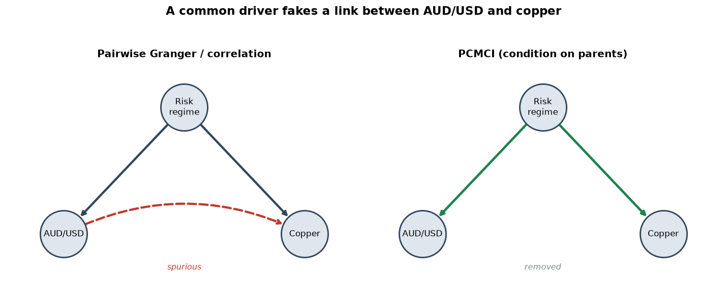
The fix your instincts reach for is to add controls. Condition on the past of every other series so the common drivers get accounted for. That is the right idea and it is the trap this whole article is about.
The dimensionality trap kills the honest test
Conditioning on the full past of every variable has a name in the paper: full conditional independence testing, FullCI. It is the rigorous, multivariate version of Granger causality. To test whether series i at lag tau drives series j now, you condition on the entire past of all N series up to the maximum lag, minus the one link you are testing.
$$ X^{i}_{t-\tau} \perp\!\!\!\perp X^{j}_{t} \;\big|\; \mathbf{X}^{-}_{t} \setminus \{X^{i}_{t-\tau}\} $$
Read it as: driver at a lag is independent of the target now, given the past of everything else. The conditioning set is the whole history of the system, so the test controls for every common driver and indirect path you have measured. That is exactly what you wanted. The problem is the size of that conditioning set. With N series and a maximum lag of tau_max, you are conditioning on roughly N times tau_max minus one variables in a single test.
Work the number a quant would actually hit. Thirty instruments, five daily lags, so the conditioning set is 30 times 5 minus 1, which is 149 variables. If you have one trading year of clean daily data, call it 250 observations, you are fitting a relationship with 149 controls on 250 points. The degrees of freedom are almost gone, and the effect size you are trying to detect gets diluted by every irrelevant control you throw in. In the climate example the true link Nino to British Columbia had a FullCI partial correlation of about 0.1 with a p-value of 0.037 in the bare bivariate case. Add one variable that is itself driven by Nino and the effect size drops to 0.09, and the link is detected in only 53% of realizations. Add six more autocorrelated series and detection power falls to 40%. The link never changed. The test just went blind.
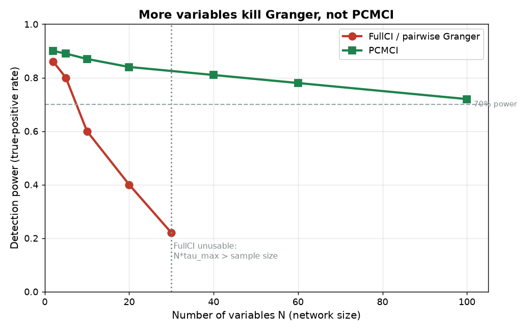
The pattern is brutal and monotone. FullCI holds about 80% power at five variables, drops to 40% at twenty, and simply cannot run once N times tau_max exceeds your sample size. So you are stuck between two bad options: bivariate Granger that reports spurious links, or full-conditioning Granger that goes deaf the moment the network gets interesting. That is the dilemma, and adding more data is rarely the escape because markets are non-stationary and last year's regime is not this year's.
PCMCI step one: find the few parents that matter
The way out is to stop conditioning on everything and condition only on the variables that actually matter, the direct causes. Causal discovery theory gives you a clean result: the parents of a variable, its direct causal drivers, are a sufficient set to condition on. You do not need the whole history. You need the handful of series that genuinely drive the target.
PCMCI's first stage, called PC1, is a condition-selection algorithm that hunts down that handful. It starts by assuming every lagged variable is a potential parent, then iteratively strips out the ones that wash out. First pass removes anything with no unconditional association at all. Second pass removes anything that becomes independent once you condition on the single strongest driver found so far. Third pass conditions on the two strongest, and so on, until nothing more drops. What survives is a short list of likely parents.
The design choice that matters here is that PC1 runs with a deliberately loose significance level. You want it to over-include, to keep the real parents even at the cost of dragging in some false ones, because the next stage cleans up false positives. In the experiments, PC1 still recovered more than 80% of true parents even at 100 variables. At that size more than 80% of the conditions it selected were false positives, but the list was still a tiny fraction of the 500 lagged variables FullCI would have conditioned on. You traded a saturated 149-control regression for a lean five-control one, and that is where the power comes back.
PCMCI step two: MCI conditions on both ends
Getting the conditioning set small is half the fix. The other half is the false-positive problem that autocorrelation creates, and this is the part plain PC-style algorithms get wrong. The momentary conditional independence test, MCI, tests the link from driver to target while conditioning on two parent sets at once: the parents of the target, and the parents of the driver.
$$ X^{i}_{t-\tau} \perp\!\!\!\perp X^{j}_{t} \;\big|\; \mathcal{P}(X^{j}_{t}) \setminus \{X^{i}_{t-\tau}\},\; \mathcal{P}(X^{i}_{t-\tau}) $$
Read it as: driver at a lag is independent of the target now, given the parents of the target and the parents of the driver. Conditioning on the target's parents is what kills spurious and indirect links, the same job FullCI was doing, but now with five controls instead of 149. Conditioning on the driver's own parents is the extra piece, and it is there to soak up autocorrelation. A strongly autocorrelated series carries information about its own past, and if you do not control for that, a mechanically persistent series will look like it is causing things it is not. Adding the driver's parents to the conditioning set corrects the false-positive rate back to the nominal level, even when both series are heavily autocorrelated.
Work it against the climate case. The bare FullCI link Nino to British Columbia had effect size 0.1 that decayed to 0.09 and then vanished into 40% power as controls piled up. MCI, conditioning only on the few real parents, holds the partial correlation at about 0.10 with a p-value of 0.036 in all three variants, and detection power stays above 80% even in the high-dimensional case. Same link, same effect size, no collapse. For finance this is the whole ballgame: it means a causal link you find in a two-asset study does not evaporate when you expand the analysis to the full basket, which is precisely what happens with FullCI. Autocorrelation is not a corner case here either. Volatility clustering, momentum, and slow-moving macro series make financial data some of the most autocorrelated you will ever test, so the FDR control that MCI buys is not a nicety, it is the difference between a network you can act on and one that is mostly artifacts.
Effect size is causal strength, not correlation
There is a bonus in MCI that changes how you read the output. The MCI statistic is not just a pass-fail flag, it is an estimator of causal strength, and it behaves far better than correlation as a ranking tool. The paper defines the standardized causal effect of a link with coefficient c as follows.
$$ \text{causal strength} = \frac{|c|}{\sqrt{1 + c^{2}}} $$
Read it as: the true strength of a link scales with its coupling coefficient, squashed into a bounded range. Work two: a weak link with c equal to 0.15 has a causal strength of 0.15 divided by the square root of 1.0225, which is 0.148. A strong link with c equal to 0.5 has strength 0.5 over the square root of 1.25, which is 0.447. Now the point. When you fix every link in a synthetic network to the same c and measure how three methods report it, correlation is all over the map, spanning nearly zero to high values for links that are all equally causal. It is essentially unrelated to causal strength, which is why a correlation-ranked list of drivers is nearly worthless. FullCI partial correlation is tighter but systematically smaller than the truth. MCI sits right on the true causal-strength line.
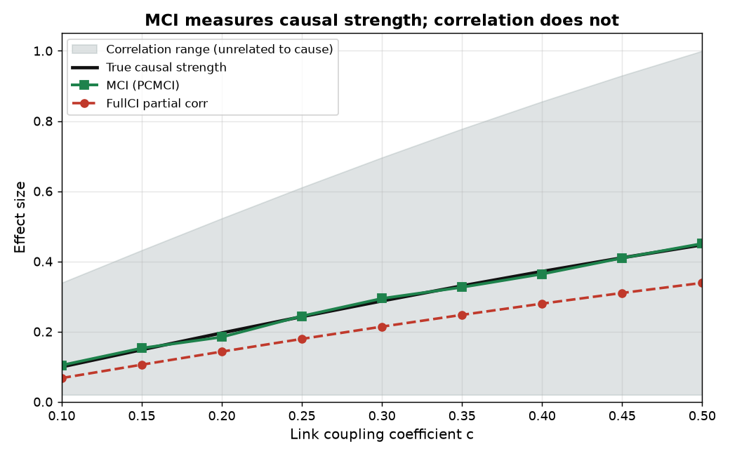
For a quant this means the MCI value on each surviving edge is a rankable number. You can say the rate-to-currency link is genuinely stronger than the equity-to-currency link and mean it, rather than mistaking a big correlation for a big cause. The old article "Regularization from First Principles" made the case that Lasso is the standard tool for picking a few active drivers out of many. Runge's experiments put Lasso in the same test, and the sting is in the worst case: even at ten variables Lasso constantly overlooks a slice of the true links, while PCMCI kept detection power above 70% on 99% of links. Lasso optimizes prediction, not causal significance, and the gap shows up exactly where you care.
Pick the independence test to match your data
PCMCI does not hard-code how it measures dependence. Both PC1 and MCI plug into any conditional independence test, and the paper works three. Linear partial correlation, ParCorr, is fast and assumes linear additive noise, the right default when you believe your relationships are roughly linear. GPDC uses Gaussian process regression with a distance-correlation test on the residuals, which catches nonlinear links with additive noise at the cost of speed. CMI is a fully non-parametric conditional-mutual-information test built on a k-nearest-neighbor estimator, and it catches almost any dependence structure, including the messy nonlinear couplings that live in stressed markets. The old article "Mutual Information as a Regime / Noise Filter" already made the case for mutual information over correlation when relationships bend; CMI is that idea wired into a causal discovery engine.
The tradeoff is the usual one. The more general the test, the more data it needs. GPDC and CMI have lower power than ParCorr on genuinely linear relationships at small samples. So the honest workflow is to run ParCorr first, and only reach for GPDC or CMI when you have reason to believe the linear test is missing a nonlinear driver and you have the sample size to support the switch.
What PCMCI does not promise
Keep the skepticism pointed at the method too. PCMCI rests on assumptions that finance violates more often than climate does. Causal Sufficiency assumes every common driver is in your dataset. If the true regime variable, a central-bank stance or a liquidity shock, is not one of your series, PCMCI will still hand you a confident network and some of its edges will be that missing driver in disguise. The word causal here is always relative to the variables you included, nothing more.
Two more limits. PCMCI as described handles time-lagged links only, where the arrow of time settles direction; it does not resolve contemporaneous, same-bar causality, which is where a lot of high-frequency action lives. And observational noise degrades it: the paper found noise up to 25% of the dynamical noise standard deviation had only minor effects, but at noise levels comparable to the signal the false-positive control breaks because common drivers stop being detectable. Market data is noisy, so treat a PCMCI network as a hypothesis generator that narrows hundreds of candidate drivers to a testable few, not as a finished truth. The one asymmetry worth trusting: a link PCMCI fails to find is more believable as a genuine non-link than a link it finds is as a genuine cause, because absence of a detectable relationship rests on weaker assumptions than presence.
KEY POINTS
- Pairwise Granger across many instruments reports mostly spurious links, because markets are full of common drivers, heavy autocorrelation, and indirect chains that a two-series test cannot see.
- The obvious fix, conditioning on the full past of every series (FullCI), controls spurious links but collapses in power. Thirty instruments at five lags means 149 controls in one test; power fell from 80% at five variables to 40% at twenty and became unusable once controls exceeded the sample.
- PCMCI stage one, PC1, selects a short list of likely parents by iterative conditioning, deliberately over-including to protect real drivers. It recovered over 80% of true parents even at 100 variables.
- PCMCI stage two, MCI, tests each link conditioning on the parents of both the target and the driver. The target's parents kill spurious and indirect links with a handful of controls instead of 149; the driver's parents soak up autocorrelation and restore correct false-positive control.
- MCI is an estimator of causal strength, so its value ranks links honestly. Correlation is nearly unrelated to true causal strength; FullCI understates it; MCI tracks it. Even at ten variables Lasso overlooked links that PCMCI caught above 70% power on 99% of links.
- The dependence test is pluggable: ParCorr for linear and fast, GPDC and CMI for nonlinear at the cost of sample size. Run ParCorr first, escalate only with evidence and data.
- The assumptions bite in finance: Causal Sufficiency needs every common driver in the dataset, the method resolves lagged links only, and it degrades under signal-scale noise. Treat the output as a hypothesis generator, and trust an absent link more than a present one.
References
- Mathematical Techniques in Financial Markets - Don Mak (Amazon)
- Cycle Analytics for Traders - John Ehlers (Amazon)
- Detecting causal associations in large nonlinear time series datasets (Detecting causal associations in large nonlinear time series datasets)
A note on AI. The ideas, research, analysis, and conclusions in this article are my own. I use AI tools to help with editing and wordsmithing, because English is not my first language, and I am not shy about that. AI-generated ideas and AI-assisted writing are not the same thing: the first is empty slop from a generic prompt, the second is a tool for communicating years of real research more clearly. Judge the work by its substance, not by whether software helped polish the prose.