8.7 Mutual Information as a Regime / Noise Filter
Mutual information measures whether the next move is connected to the last few or just noise. Volatility can't see the difference; MI gates your system on when structure is present and off when it drains away.
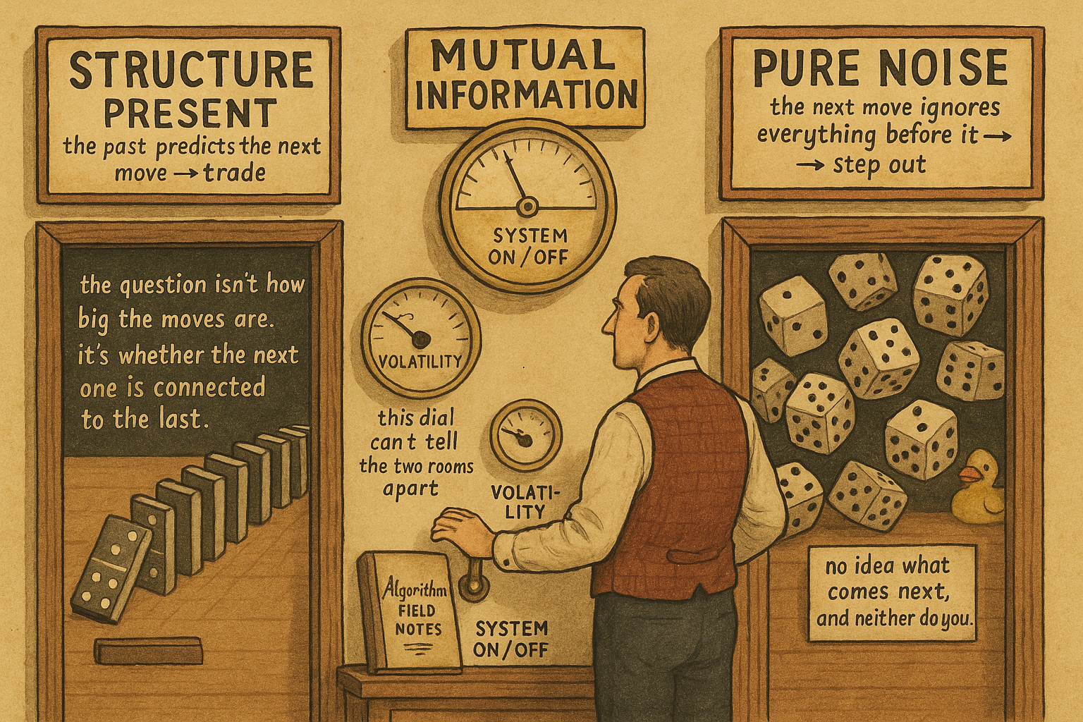
Entropy from the old article "Entropy as a Market Choppiness Gauge" tells you whether the recent tape is choppy or structured, but it answers a one-sided question: how surprising is the next move on its own. It never asks whether the next move is connected to what just happened. Mutual information closes that gap. It measures how much knowing the recent pattern of price changes tells you about the direction of the very next one, and that is exactly the quantity a trading system lives or dies on. When recent direction is statistically tied to the prior pattern, your rules have something to grip. When the tie goes to zero, the next move is independent of the last few, the noise the old article "Noise Is Not Volatility" described has taken over, and the honest call is to pull out of the market.
Two quantities, one relationship
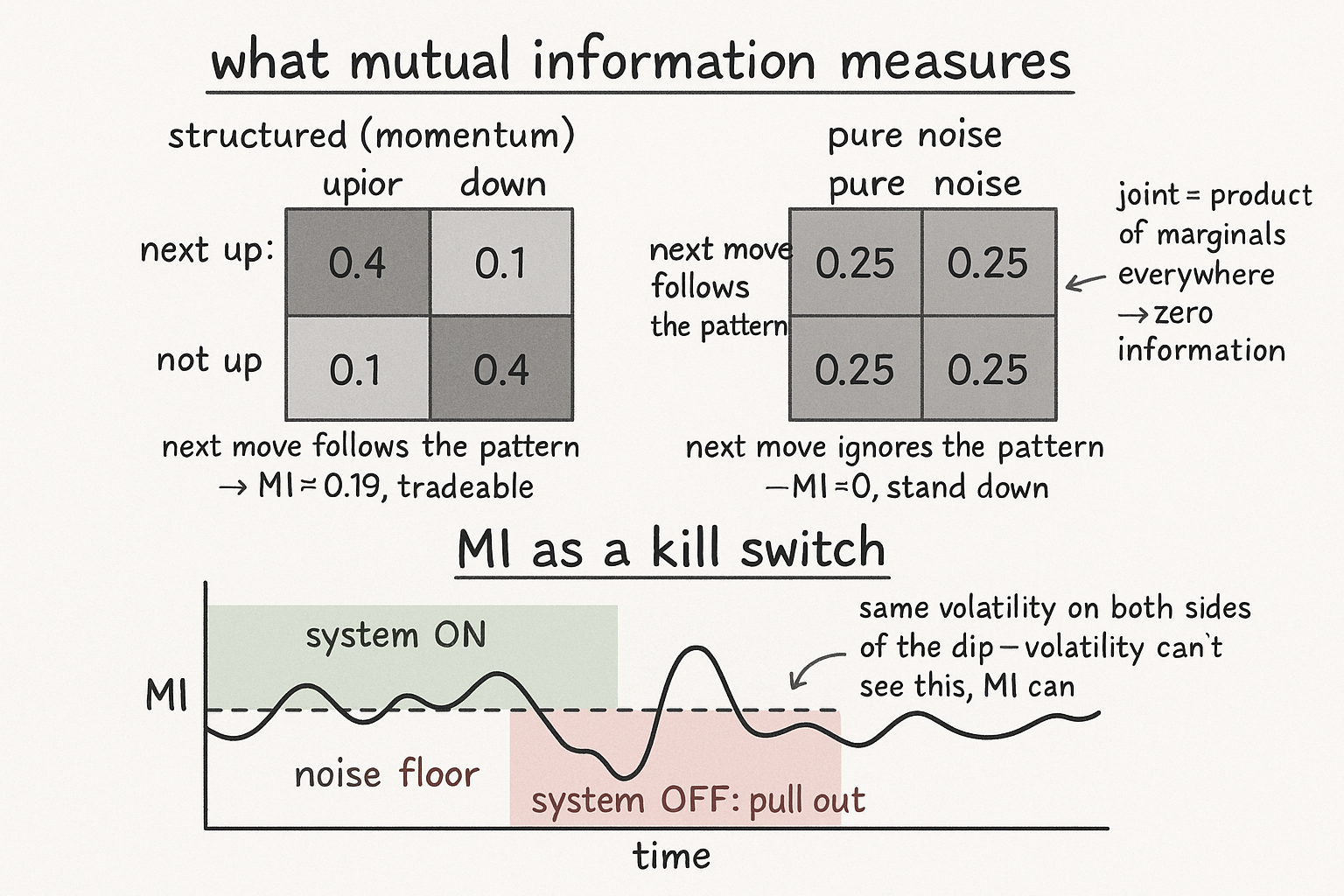
Mutual information is a general measure of how related two discrete quantities are, and the build here picks the two that matter for a trader. The first quantity is the direction of the most recent price change, a single bit: did the last bar close up or not. The second quantity is the arrangement of the prior recent moves, the same up-or-down word from the choppiness gauge, one of B possible bins. Mutual information asks how much the recent direction and the prior pattern share. If up almost always follows the pattern up-up and down almost always follows down-down, the two are tightly linked and there is momentum to trade. If the recent direction lands the same way no matter what preceded it, they share nothing.
$$ \text{MI} = \sum_{b=1}^{B} \left[ p(0,b)\,\log\frac{p(0,b)}{p(0)\,p(b)} + p(1,b)\,\log\frac{p(1,b)}{p(1)\,p(b)} \right] $$
Read it as a comparison between what happens and what would happen by chance. The index b runs over the B prior-pattern bins, the labels 0 and 1 mark the recent direction (not-up and up), and p(d,b) is the joint probability of seeing direction d together with pattern b. The marginals are the standalone odds: p(d) is how often the recent move is up or not regardless of the pattern, and p(b) is how often pattern b shows up regardless of what came next. The ratio inside each log is the tell. If direction and pattern were independent, the joint p(d,b) would equal the product p(d) times p(b), the ratio would be 1, the log would be 0, and the whole sum would collapse to zero MI. Every bit the joint pulls away from that product is structure, and MI adds it all up.
The marginals are not free parameters, they fall out of the joint table.
$$ p(0) = \sum_{b=1}^{B} p(0,b), \qquad p(1) = \sum_{b=1}^{B} p(1,b), \qquad p(b) = p(0,b) + p(1,b) $$
Sum the joint across patterns to get how often each direction occurs, and sum across the two directions to get how often each pattern occurs. Everything comes from one count table over the window: tally how often each pattern was followed by an up versus a not-up, divide by the total, and the rest is arithmetic.
A worked number
Take the simplest case, a prior pattern that is just the single previous move, so two bins, down or up, and pair it with the next move. Suppose over the window the joint probabilities come out as up-then-up 0.4, down-then-up 0.1, up-then-down 0.1, down-then-down 0.4. The market is showing momentum: a move tends to repeat. The marginals are all 0.5, since up-now totals 0.5 and up-prior totals 0.5. Plug in with natural logs. Each of the two heavy cells contributes 0.4 times the log of 0.4 over 0.25, and 0.4 over 0.25 is 1.6, whose log is about 0.47, so each heavy cell adds about 0.188. Each light cell contributes 0.1 times the log of 0.1 over 0.25, and 0.1 over 0.25 is 0.4, whose log is about minus 0.92, so each light cell subtracts about 0.092. The sum is roughly 0.188 plus 0.188 minus 0.092 minus 0.092, about 0.19 nats of mutual information: real, tradeable structure.
Now flatten it to pure noise. Make all four cells 0.25, meaning the next move is a coin flip no matter what came before. Every joint equals the product of its marginals, 0.25 equals 0.5 times 0.5, every ratio is 1, every log is 0, and MI is exactly zero. Same volatility, same average move size, but the link between past and future is gone. That zero is the signal to stand down.
Why this beats a volatility reading
The old article "Noise Is Not Volatility" made the case that how far price travels and how much of that travel survives as net direction are two different things, driven independently. Mutual information is the second of those measured directly. A market can double its volatility, throw bigger bars, and keep MI exactly where it was, because the bigger moves still follow the same patterns. Another market can keep volatility flat while MI drains to zero, the moves staying the same size but losing all connection to what preceded them. A volatility gauge cannot tell these apart; it reports the size of the bars and stays silent on whether they are predictable. MI reports the predictability and stays silent on the size, which is the half a trader actually needs to know whether the edge is live.
It also catches what linear tools miss. The old article "Entropy as a Market Concept" pointed out that a series with zero linear autocorrelation can still be predictable through nonlinear dependence, and MI does not care whether the relationship is linear. If the next direction depends on the prior pattern in any way, even one a correlation coefficient reads as zero, MI sees it, because it compares full joint probabilities against the independence baseline rather than fitting a straight line. The price is a harder estimate that needs more data to pin down than a correlation does, which is why the window has to be long enough to fill the bins.
Using it as a kill switch
Treat MI as a go or no-go gate on whatever rule you already trust, not as the rule itself. Compute it on a rolling window, and when it sits comfortably above zero the structure your system was built on is present, so let the system run. When MI decays toward zero the market has gone to noise, the next move has come unhooked from the recent ones, and the right move is to cut size or step out until it recovers, exactly the "pull out of the market" call this indicator exists to make. The noise level of markets rises and falls over time, so this is not a one-time check; it is a continuous read on whether conditions still match the ones your edge was measured in.
Two cautions keep it from lying to you. First, MI is always non-negative and any finite sample produces a small positive value even from genuinely independent data, because random counts never land exactly on the independence product, so a tiny MI is indistinguishable from zero and you should set your floor above that sampling-noise level rather than at a literal zero. Second, MI measures that a relationship exists, not what it is or which way it points; a high reading on a momentum window and a high reading on a mean-reversion window look identical, so MI tells you the edge is present and something else has to tell you how to take it. And as with entropy, every reading is a window average, so it lags the regime change that triggered it, and you cannot fix that by shrinking the window without starving the bins and turning the estimate into noise of its own.
KEY POINTS
- Mutual information measures how much the prior pattern of price moves tells you about the direction of the next one, the exact quantity a system needs: pair the recent direction (up or not, one bit) with the prior up-or-down word (one of B bins).
- The formula sums, over every cell of the joint table, the joint probability times the log of joint over the product of marginals; when direction and pattern are independent the joint equals that product, every log is zero, and MI collapses to zero.
- Worked case: a momentum window (up-up and down-down at 0.4, off-diagonals at 0.1) gives about 0.19 nats of structure, while flattening every cell to 0.25 gives exactly zero, same volatility but no link between past and future.
- It is the predictability half of the old article "Noise Is Not Volatility" measured directly: volatility can double while MI holds, or stay flat while MI drains to zero, and a volatility gauge cannot tell those apart.
- It catches nonlinear dependence a correlation coefficient reads as zero, the point the old article "Entropy as a Market Concept" raised, because it compares full joint probabilities to the independence baseline instead of fitting a line.
- Use it as a go/no-go gate: above a noise floor, run the system; decaying toward zero, cut size or pull out. Set the floor above the small positive value finite samples always produce, remember MI shows that structure exists but not its direction, and accept that it lags because it averages a window.