5.52 Lead-Lag Is Multidimensional: Trade Price and OBI Predict Others' Midpoints

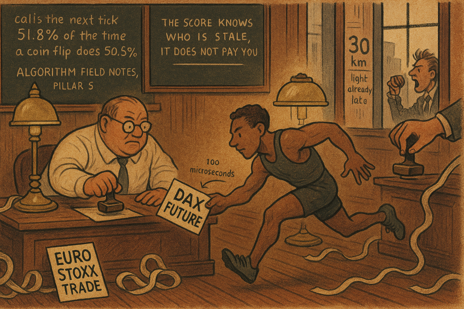
The Euro Stoxx 50 future's trade price led the DAX future's midpoint on 99% of trading days from January to June 2021, and the lag that maximized the correlation was 100 microseconds. Bender, Cestonaro, and Schmidt measure that lead on 19 Xetra and Eurex instruments, across nine microstructure series, with a lag-shifted Hayashi-Yoshida correlation: the sum of price changes whose time windows overlap, with no resampling onto a clock. Their lead-lag strength, a score that grows only when one series leads and the two series move together, sits at or above 2.29 for the top 5% of pairs when the leader is a trade price and the lagger is a midpoint. Ask the leader's last change to call the direction of the lagger's next change and the average hit rate is 51.8%, against 50.5% for a benchmark that always calls the more common direction. Hit rate and lead-lag strength correlate 0.67. The ordering of who moves first is a stable fact about a handful of related contracts. A 1.3 point edge on direction, inside a window of 100 microseconds, is a quote you cancel if you are making a market in the same data center, and a spread you donate if you try to lift it from a remote server.

What this actually is

You quote the DAX future. A trade prints in the Euro Stoxx 50 future. In this sample the DAX midpoint follows that trade, same direction, and the match peaks 100 microseconds later. Leave the resting quote and a faster participant lifts it. That pickup is the whole economic content of the paper.

The method lines up two uneven streams of trades and book updates and asks which stream's changes match the other's later changes. Nothing is forced onto a one-second grid.

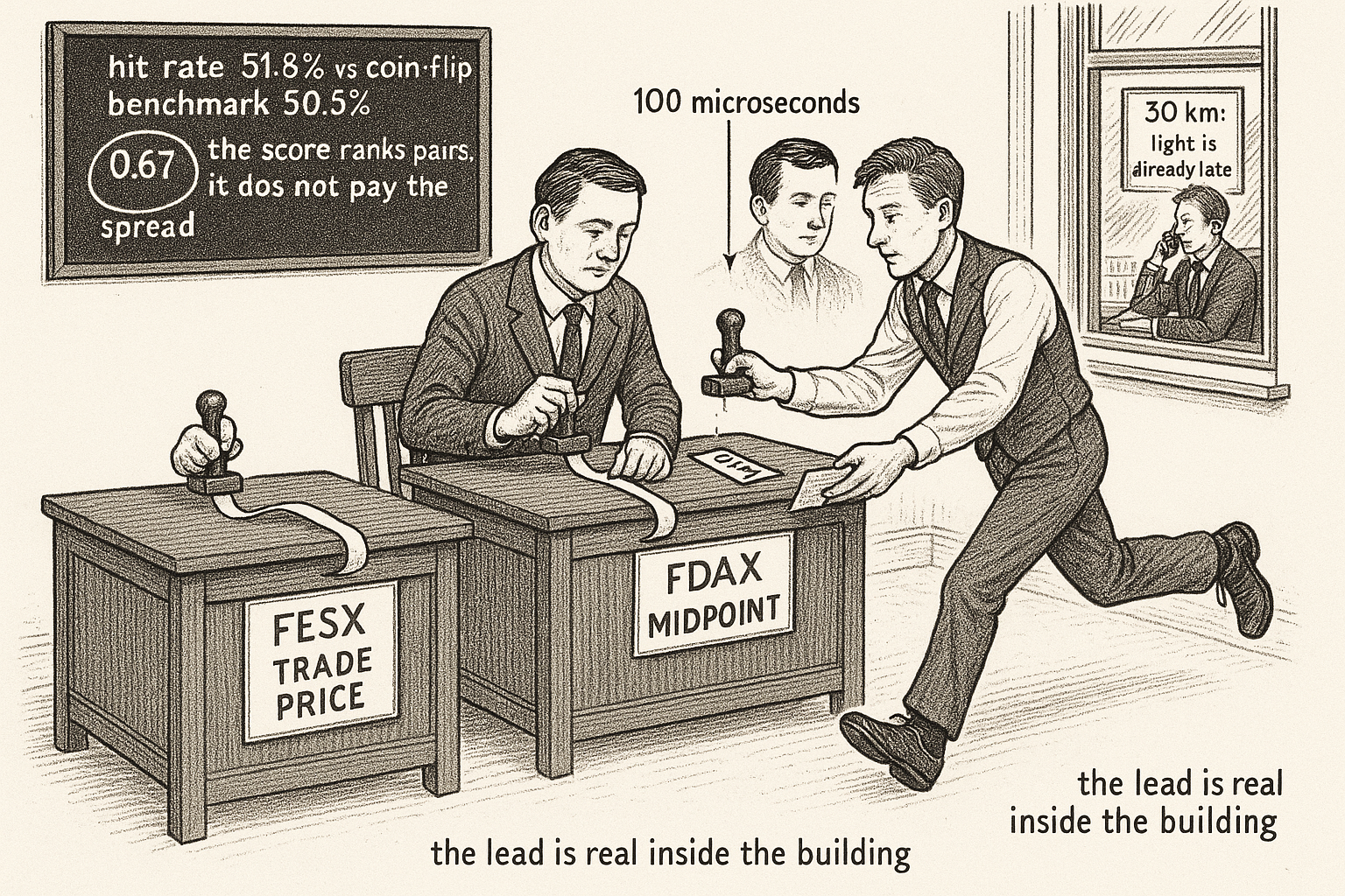
Picture two clerks in one room, each stamping a ticket only when their own book changes. The stamps do not share a metronome. Count the pairs of stamps whose time windows overlap, multiply the two price changes, and add. Then slide one clerk's clock forward by a chosen lag and count again. The lag where the sum peaks is how far ahead that clerk is.

If the claim holds, you read the leader's trade before you leave a resting order in the lagger, or you widen the quote by enough to pay for being picked off. Treating the 51.8% hit rate as a signal you can take from outside the matching engine means you cross a spread to bet a coin flip that wins an extra 1.3 times in a hundred, on a clock your connection cannot see. In vacuum, light covers 30 kilometers in 100 microseconds. A desk outside that radius is already late when the message arrives.

Overlapping increments, not a resampled clock

Two series that tick at different times still have a correlation, and forcing them onto a fast clock drives that correlation to zero. Downsample both to one-minute bars and you can run a regression, which is what the older lead-lag papers did, and what the old article "Lead-Lag Relationships in Global Markets" does with lagged cross-correlation on a regular clock. Push that same grid down toward the speed of the trades and the correlation shrinks toward zero even when the two prices are the same price. Epps documented that bias in 1979. Interpolation manufactures the bias.

Hayashi and Yoshida skip the grid. Split each series into the intervals between its own observations. Multiply the change on an interval of the first series by the change on an interval of the second only when the two intervals overlap, add every such product, and divide by the square root of the summed squared changes of each series. Hoffmann, Rosenbaum, and Yoshida then slide the second series by a lag ell before testing the overlap. A positive ell lays the second series' earlier changes on top of the first series' later changes, so a large correlation at a positive ell means the second series leads.

$$ \hat{\rho} = \frac{\sum_{i,j} \Delta X(I_i)\, \Delta Y(J_j)\, \mathbf{1}\{I_i \cap J_j \neq \emptyset\}} {\sqrt{\sum_i [\Delta X(I_i)]^2 \; \sum_j [\Delta Y(J_j)]^2}} $$ $$ \hat{\rho}(\ell) = \frac{\sum_{i,j} \Delta X(I_i)\, \Delta Y(J_j)\, \mathbf{1}\{I_i \cap (J_j + \ell) \neq \emptyset\}} {\sqrt{\sum_i [\Delta X(I_i)]^2 \; \sum_j [\Delta Y(J_j)]^2}} $$

Read the first line as an overlap correlation. Delta X on interval i is the price change of series X between two of its own prints, in price points. The indicator is 1 when that interval shares any time with interval j of series Y, and 0 otherwise. The denominator rescales by each series' own size, so the ratio is unitless. The second line is the same sum after every Y interval has been moved by ell seconds. Positive ell: Y leads X. Negative ell: X leads Y.

Worked toy, not a market. X rises 4 points from 0 to 10 seconds and 3 points from 10 to 20 seconds. Y rises 4 points from 1 to 2 seconds and 3 points from 11 to 12 seconds. Each X interval overlaps exactly one Y interval, the products are 16 and 9, the numerator is 25, and each series' summed squares are 25, so the correlation at lag zero is 25 over 25, which is 1. Slide Y forward by 15 seconds and the only surviving overlap is the 3-point X change with the shifted 4-point Y change. The numerator falls to 12 and the correlation falls to 12/25, which is 0.48. Slide Y backward by 15 seconds and nothing overlaps, so the correlation is 0. Y's earlier move lines up with X's later move. Y leads. The same arithmetic, run on nanosecond stamps, is the whole estimator.

Two design choices bound what that number can mean. The authors keep a measure only at times when a trade prints, the same filter Hoffmann and Huth used for prices. An order-book imbalance that changes between trades never enters the sum. And they estimate one curve per instrument pair, per measure pair, per day, on a fixed menu of 35 lags: 17 leads, 17 lags, and the contemporaneous point, from 10 microseconds out to 60 seconds. Nineteen names, nine measures, and cross-name pairs only (19 times 18 times 81) give 27,702 series pairs. Times 124 sessions, that is 3,435,048 daily curves. They drop a day when the two series share fewer than 100 overlapping intervals, which leaves 2,119,921 curves, 61.7% of the total. They call that about 61%. Four pairs, all involving the silver note, fail a 21-day minimum and leave the sample.

A strength score that ignores fake asymmetry

The lag of the peak is a thin summary of the curve, and the lead-lag ratio is a misleading one. The maximizing lag records a direction and ignores every other point. Huth and Abergel's lead-lag ratio keeps the whole curve: summed squared correlations on positive lags, divided by the same sum on negative lags. Above 1, the shifted series leads. A ratio of 4 can come from correlations of 0.4 or from correlations of 0.0004.

$$ LLR = \frac{\sum_{\ell>0} \hat{\rho}(\ell)^2}{\sum_{\ell<0} \hat{\rho}(\ell)^2} $$ $$ LLS = \begin{cases} \left(\dfrac{\sum_{\ell>0}\hat{\rho}(\ell)^2}{\sum_{\ell<0}\hat{\rho}(\ell)^2}-1\right) \dfrac{100}{n_L}\sum_{\ell} \hat{\rho}(\ell)^2 & \text{if that ratio}\ge 1,\\[1em] \left(\dfrac{\sum_{\ell<0}\hat{\rho}(\ell)^2}{\sum_{\ell>0}\hat{\rho}(\ell)^2}-1\right) \dfrac{-100}{n_L}\sum_{\ell} \hat{\rho}(\ell)^2 & \text{otherwise.} \end{cases} $$

Read the lead-lag ratio as a comparison of two areas under the curve. Read the lead-lag strength as that comparison, minus one, multiplied by 100 times the average squared correlation across the grid. n_L is the number of lags on the grid, here 35, counting lag zero. The sum in the last factor runs over every lag, including zero. Positive strength means the shifted series leads, and the absolute value is the same if you swap which series you shift. The authors' typeset equation is missing the opening parenthesis in front of the ratio, so the line as printed does not parse. The card is the grouping their prose describes, with that parenthesis restored.

Their own footnote is the reason the ratio is not enough. Set every positive-lag correlation to 0.001 and every negative-lag correlation to 0.0005. With 17 lags on each side the summed squares are 17 times 0.000001 and 17 times 0.00000025, and the ratio is 4. A lead-lag ratio of 4 sounds like a strong lead. The correlations are noise. Put lag zero at 0, which the footnote leaves unspecified, and the lead-lag strength is (4 minus 1) times (100/35) times 0.00002125, which equals 0.000182. Swap which series is shifted and the strength is minus 0.000182. The same absolute value, opposite sign, which the ratio does not give you: the swapped ratio is 0.25, not minus 4. In the real sample the 95th percentile of strength for trade price leading midpoint is 2.29, about 12,600 times the footnote's fake lead. The strength stays near zero when the curve is flat and tiny, and it gets large only when the curve is both lopsided and tall.

Trade price and imbalance lead; quoted depth does not

Trade prices and best-quote imbalance lead other names' midpoints. Quoted spread, volume, and resting depth do not. The authors rank measure pairs by the 95th percentile, across instrument pairs, of the daily peak correlation and of the lead-lag strength. That percentile is the value the best 5% of pairs clear, so a quiet cell means even the strongest pairs in that cell are quiet.

Price against price is the loud cell. Five percent of pairs have a peak midpoint correlation of 0.88 or higher, and the midpoint-against-trade-price cell is 0.76 on the same percentile. Quoted spread, traded volume, size at the best quotes, and size at the ten best levels sit near 0.01 to 0.05 against the other series. Two off-diagonal leads survive. Trade price of one name leading the midpoint of another has a 95th-percentile strength of 2.29. Order-book imbalance (OBI) at the best quotes, the euro amount on the bid minus the euro amount on the ask divided by their sum, leading the other name's midpoint has a 95th-percentile strength of 0.55. The reverse, midpoint leading future imbalance, is about zero. Transaction-price volatility leading midpoint volatility is the third pair they keep, with a 95th-percentile peak correlation of 0.21 or higher. They then study one pair from each family: trade price into midpoint, imbalance into midpoint, and transaction-price volatility into midpoint volatility.

$$ OBI_t = \frac{P^{bid}_t Q^{bid}_t - P^{ask}_t Q^{ask}_t} {P^{bid}_t Q^{bid}_t + P^{ask}_t Q^{ask}_t} $$

Read it as a signed fraction of euro depth at the inside. Prices are in currency per unit, sizes are in units, both products are in currency, and the ratio is unitless, between minus 1 and 1. Worked book: bid 100.00 for 500, ask 100.10 for 200. Euro bid is 50,000, euro ask is 20,020, and the imbalance is 29,980 / 70,020, which is 0.428. The share-count version used in the old article "The Worst-Kept Secret: Imbalance Is the MM's Optimal Response, Not Alpha", (500 minus 200) over (500 plus 200), is 0.429. At the inside quote the two agree. The lead this paper finds is the object that article warns you about. Imbalance is the market maker's reply to a price she already expects, so a lead from one name's imbalance into another's midpoint can be two books answering the same latent price. Cont, Cucuringu, and Zhang document the same cross-name pattern: order-flow imbalance in one equity moves the midpoint of another.

The instrument map is a map of shared underlyings. Volkswagen and Daimler, both autos, correlate with each other and with the DAX and Euro Stoxx futures and ETFs. Pair either of them with SAP and the correlation drops. The Euro Stoxx future is the dominant leader: its trade price leads the midpoint of every stock and equity future in the sample, and the strength keeps the same sign on 99% of days, which is the three-star mark in their figure. The Swiss future does the same. The DAX future and the Mini-DAX future lead the three DAX stocks, and the stocks lead them back, with SAP, the heaviest DAX weight, the strongest and most persistent of those reverse leads. That two-way result is what the law of one price says you should see. A DAX constituent trade moves the index future because the index is the constituents. An index-future trade moves the constituent because both are the same bet.

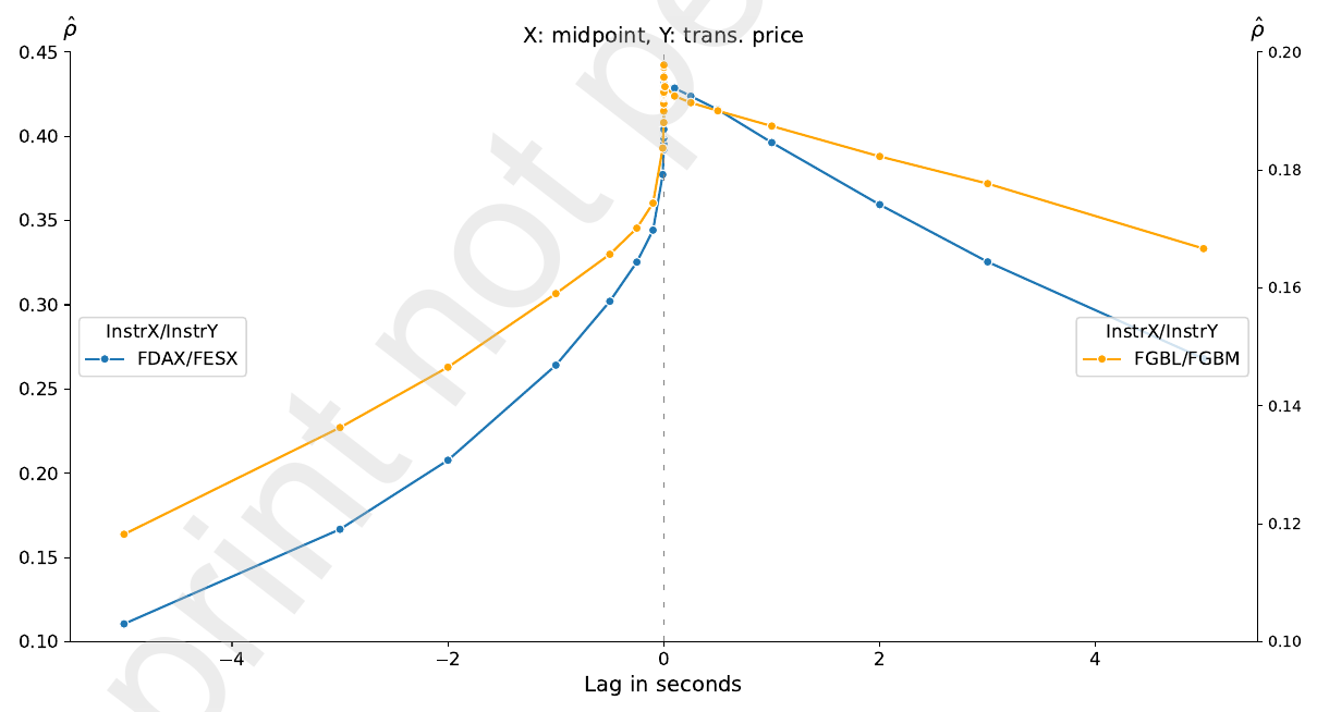
On the zoomed curve the Euro Stoxx trade price leads the DAX midpoint by 100 microseconds, and the Bobl trade price leads the Bund midpoint by the same 100 microseconds. The curve stays elevated for several seconds away from zero and decays faster when the lag is negative. The peak itself is a tenth of a millisecond. The authors, citing Deutsche Boerse, put the fastest members' reaction under 3 microseconds, so a colocated trader can act many times inside that 100 microsecond lead. Budish, Cramton, and Shim's stale-quote sniping is this picture with a name on it: the fast trader hits the DAX quote that has not yet moved to the Euro Stoxx trade.

Imbalance is slower, and one-directional. The curves fall to about zero after five to ten seconds, imbalance leads midpoint, and midpoint does not lead imbalance. Daimler's imbalance leads the DAX future's midpoint by one second and Volkswagen's midpoint by two seconds. One second is a different operational problem from 100 microseconds. A fast quoter can see it. The futures-versus-futures trade-price lead is for members who already live inside the exchange's latency budget.

Volatility splits by how often the name trades. The DAX future's transaction-price volatility leads the Mini-DAX future's midpoint volatility by one millisecond. Between the two bitcoin notes the lead is two seconds, and the correlation only falls from 0.461 to 0.446 at a ten-second lead. The thinner note, 21XB, trades about 2.0 million euros a day with 77 seconds between trades. The thicker one, BTCE, trades about 26.6 million euros a day with 21 seconds between trades. The correlation cannot die in ten seconds when the next print may not exist yet. The authors searched every pair, with no pre-chosen fundamental link. The pairs that light up share an underlying or a risk factor.

Liquid names lead, until you leave equities

The same pair's lead does not track that day's volume, and the more active name leads only inside equities. Bin each pair's days by the combined rank of the two names' volume, by the gap between their trades, and by midpoint volatility. The lead-lag strength inside those bins barely moves. The same null shows up for turnover per trade, relative spread, and the share of trades that hit past the first price level. The day-to-day wobble in the strength is not the day's liquidity.

The cross-section is where the old equity result shows up, and then breaks. Huth and Abergel, on midpoints, found that the name with more trades and a tighter book tends to lead. Here the authors regress daily strength on the log of an indicator ratio, indicator of the midpoint name over indicator of the shifted name, one indicator at a time so the liquidity proxies do not fight each other. A negative coefficient means the shifted name's lead gets stronger as its own indicator rises relative to the other name. They print coefficients, standard errors, and adjusted R-squared in percentage points. N is 113,520 in the full sample, pooling the three measure pairs.

$$ LLS_{m,i,t} = \beta_0 + \beta_1 \log\frac{I_{X,i,t}}{I_{Y,i,t}} + \varepsilon_{m,i,t} $$

Read it as a line. The left side is the lead-lag strength for measure pair m, instrument pair i, day t. The ratio inside the log is a liquidity or volatility statistic of the midpoint name divided by the same statistic of the shifted name, unitless. Beta-one is the change in strength for a one-unit rise in that log, which multiplies the ratio by e, about 2.718.

On average turnover per trade, the equity subsample prints beta-one of minus 18.0 with a standard error of 0.9 and an adjusted R-squared of 0.8%. Add dummies for whether each leg is a stock, an equity future, or an equity ETF and the slope goes to minus 25.3 (standard error 1.7) while the adjusted R-squared goes to 11.0%. The slope has the sign the equity literature wants: more turnover on the leader, stronger lead. The fit says the turnover ratio accounts for under one percent of the variation, and knowing the instrument types accounts for the jump to 11%. In the full sample the same slope is minus 2.4 (0.1) with an adjusted R-squared of 0.1%, and minus 6.3 (0.5) with 13.3% once asset-class dummies enter. The equity slope is an equity fact. Bonds and notes dilute it.

The sign is not even stable inside equities. On intertrade duration, seconds between trades, the equity slope is minus 1.2 (0.3) with no dummies and plus 10.2 (1.1) with them. The positive sign matches "the name that trades more often leads," because a higher duration ratio means the shifted name's trades are closer together. That sign shows up once the instrument-type dummies are in the regression. On midpoint volatility the equity slope is plus 17.3 (0.9) without dummies, the less-volatile name leading, and plus 1.9 (2.0) with dummies, a standard error larger than the coefficient. The volatility story dies as soon as you know what you paired.

The bond futures are the counterexample you can see without a regression. The Bund trades about 92.8 million euros a day, with 0.24 seconds between trades. The Schatz trades about 18.6 million euros a day, five times less, with 3.91 seconds between trades, about 16 times less often. The Bobl sits in between, at 39.1 million euros. Trade prices of the Schatz and the Bobl lead the Bund's midpoint. The Bund does not lead them back. The less active contracts lead the most active one. Whatever you learned about leadership from stocks and equity futures, do not carry it into the bond curve. The equity subsample is 39,040 rows and the non-equity subsample is 16,787. Those do not add to 113,520. Pairs that mix a stock or equity future with a bond, a metal note, or a bitcoin note sit in the full sample and in neither subsample, which is why the full-sample slope is so much flatter.

Direction accuracy ranks the lead and does not pay the spread

A higher lead-lag strength ranks which pairs call the next change, and the average call is 51.8%. The authors average the daily strength over January through May 2021 and score June. For every pair whose average strength is positive, the shifted series is the leader. Each time the leader changes, they call the lagger's next change in the same direction when the peak correlation is positive, and in the opposite direction when it is negative. They keep only the latest leader change as the live call. Accuracy is correct calls divided by the number of changes in the lagger. The benchmark always calls whichever direction was more common for that lagger.

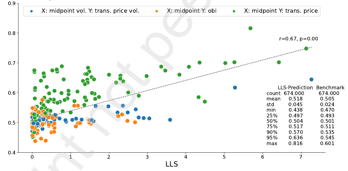
Six hundred seventy-four pairs have a positive average strength. Mean accuracy is 51.8% for the lead-lag call and 50.5% for the benchmark. The median is 50.4% against 50.1%. The 90th percentile is 57.0% against 53.5%, the 95th is 63.6% against 54.5%, and the best pair reaches 81.6% against a benchmark whose own best is 60.1%. Those two maxima need not be the same pair. The worst lead-lag call is 43.8%, worse than the benchmark's worst of 47.0%. On a dead pair, following the "leader" loses to the base rate. The correlation of 0.67 (they print a p-value of 0.00) says the strength ranks pairs. It does not say the average pair has a trade.

Restrict the scored changes to a window from half the estimated lead time to one and a half times that lead time, and the mean accuracy rises to 53.3%. The authors say the upper tenth of pairs gains another 4.1 percentage points relative to the unwindowed call. For the Euro Stoxx into DAX pair the lead time is 100 microseconds, so the window is 50 to 150 microseconds after the Euro Stoxx trade. That is the only horizon on which the improved number applies to the headline pair.

Put a spread next to the hit rate. The appendix table reports a relative quoted spread of 1.00 basis points on the DAX future and 2.56 basis points on the Euro Stoxx future. The same appendix prints the spread formula as bid minus ask, over the midpoint, which is negative on any two-sided book, while every spread in the table is positive. The formula and the table disagree. The positive table values are the ones used here. The printed sign is a typesetting error. A 51.8% call on the direction of the next midpoint change, before any queue or fee, is a 1.3 point edge over a coin flip. Crossing a 1 basis point spread to express it hands back more than the edge on a one-tick move. The paper reports no profit, no cost, and no fill model. The out-of-sample window is June 2021, one month after a five-month average, inside a single half-year on one exchange group.

The useful object is the ranking. Strength near zero, and the other series has nothing to say. Strength in the right tail, and the leader's last change calls direction well above the base rate, on a horizon equal to the lag that maximized the curve. For a market maker in the DAX future, cancel or skew when the Euro Stoxx future trades, inside a tenth of a millisecond, or widen by the spread you will donate to the member who saw it. For anyone else the 0.67 describes whose midpoint is stale.

The old article "From Intermarket Analysis to Network Momentum" wants a learned graph of who spills into whom. This sample's graph is a star with the Euro Stoxx future at the center, plus a bond-curve edge that runs from the thin contracts toward the Bund, and it is stable within these six months. The old article "Stop Using Pairwise Granger: PCMCI for Financial Causality" is the caveat on reading that star as a cause. Euro Stoxx and DAX share the European equity factor. The more active contract can print the factor first without being the parent of the other. Pairwise overlap correlation, like pairwise Granger, cannot see the common driver. It can still tell you which quote is the stale one. That is the market maker's question, and it is the only question these numbers answer.

KEY POINTS

• The Euro Stoxx 50 future's trade price leads the DAX future's midpoint on 99% of days in January to June 2021, and the Hayashi-Yoshida curve peaks at 100 microseconds. The Bobl leads the Bund by the same 100 microseconds.
• The estimator multiplies price changes whose intervals overlap, then slides one series by a lag. Resampling onto a fast clock biases the correlation toward zero, which is the Epps effect. Measures are recorded only when a trade prints, so imbalance changes between trades are invisible.
• Lead-lag strength multiplies curve asymmetry by the average squared correlation. The authors' example of correlations at 0.001 against 0.0005 produces a lead-lag ratio of 4 and a strength of 0.000182. The real 95th percentile for trade price leading midpoint is 2.29. Their typeset formula is missing an opening parenthesis; the prose version is the one used here.
• Of nine microstructure series, trade price leading another name's midpoint (strength 2.29 at the 95th percentile) and best-quote imbalance leading another name's midpoint (strength 0.55) are the price-side results. Quoted spread, volume, and depth barely correlate. Daimler's imbalance leads the DAX future by one second, not by 100 microseconds.
• More turnover and more frequent trades line up with leadership in equities, with adjusted R-squared under 1% until instrument-type dummies lift it to about 11%. The Schatz trades five times less euro volume than the Bund and leads it anyway. Day-to-day liquidity does not explain day-to-day strength.
• June 2021 direction accuracy averages 51.8% against a 50.5% base-rate benchmark, the median is 50.4%, and accuracy correlates 0.67 with lead-lag strength. The 95th percentile is 63.6%. A window around the estimated lead time lifts the mean to 53.3%. No costed P&L is reported. The DAX future's relative spread in their table is 1.00 basis points, wider than the average edge.

References

• Cross-impact of order flow imbalance in equity markets - Cont, Cucuringu, Zhang (Quantitative Finance, 2023)
• The High-Frequency Trading Arms Race: Frequent Batch Auctions as a Market Design Response - Budish, Cramton, Shim (Quarterly Journal of Economics, 2015)
• Lead-Lag Relationships in Market Microstructure - Bender, Cestonaro, Schmidt (ssrn-5043260)