3.40 Does Complexity Actually Help? (flagship)
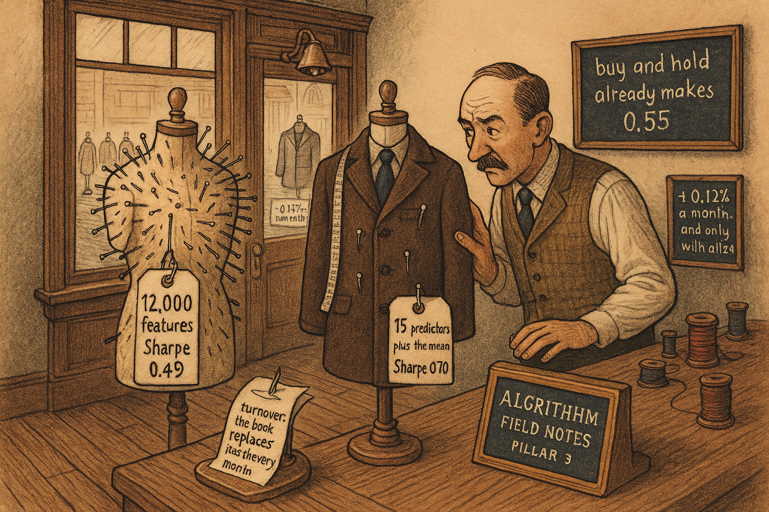
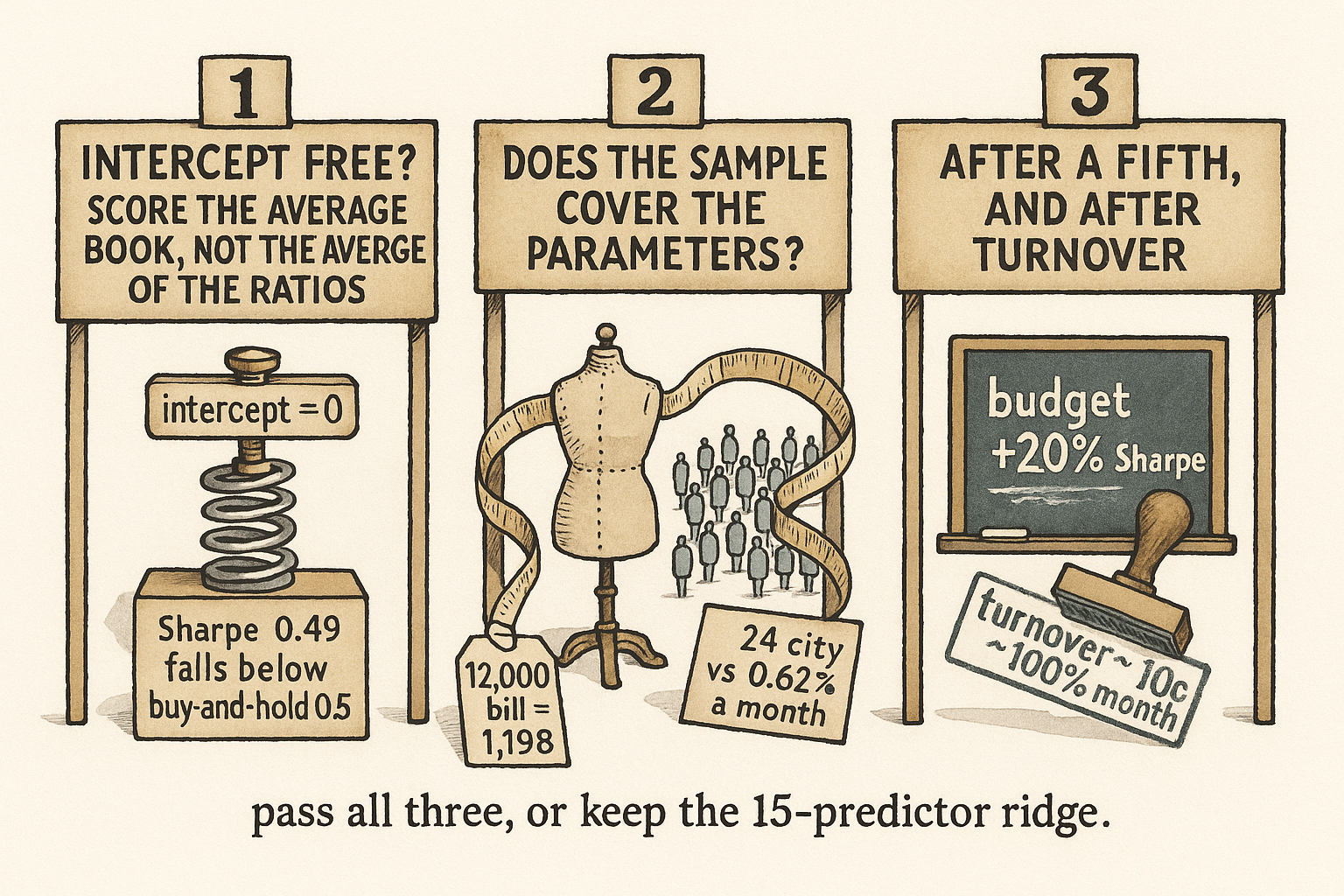
Out-of-sample Sharpe: 12,000 features score 0.49 and lose to buy-and-hold at 0.55. Complexity pays only with more data, by 0.12%/month on a global cross-section.
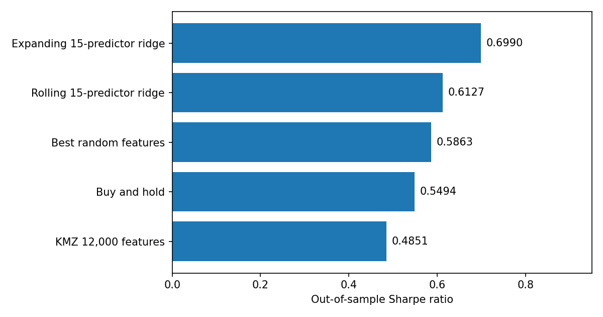
Buy-and-hold on the volatility-scaled US market earns an out-of-sample Sharpe ratio of 0.5494 from January 1940 to December 2020. The 12,000-feature timing model that Kelly, Malamud, and Zhou offer as evidence that performance rises with complexity earns 0.4851 on that same window. A ridge regression on the 15 Goyal-Welch predictors, with an intercept and a 120-month expanding window, earns 0.6990. Move the same question to a neural network and a cross-section of stocks in 24 developed markets, and the global network earns 0.74 percent a month against 0.62 percent for the same network trained region by region. Complexity helps when the sample can carry the parameters. The help is a fraction, not a multiple. The rising curve in the original paper is two choices in the plot.
What this actually is
You have a monthly decision on the S&P 500, or a long-short book across developed-market stocks, and a model with thousands of fitted weights. The S&P hands you about 120 months inside a training window. The cross-section hands you thousands of stocks in 24 countries. The method is a count. Put the number of parameters next to the number of observations, put the unconditional mean back into the regression, and only then ask whether a more flexible fit beats a short ridge or ordinary least squares.
Picture a tailor with twelve measurements of one client and a pattern that places 12,000 darts. The coat fits last year's posture. Next month the client has moved, and the extra darts are memorized noise. Give that tailor measurements from every client in 24 cities and a more flexible pattern starts to earn a small improvement in the fit.
At the desk the claim changes the build order. Add observations before adding parameters, leave the intercept unpenalized, and budget about a fifth on the Sharpe ratio before costs. Believing the headline and trading the 12,000-feature timing book means holding a 0.49 Sharpe strategy against a 0.55 buy-and-hold, before spreads. Refusing every flexible model means skipping the 0.12 percentage points a month that the global network earns over its regional twin. The two mistakes are different sizes.
Two choices, and the curve flattens
The question is whether portfolio performance rises as the model grows more complex. On this equity-premium sample, it rises only under two restrictions, and both of them are choices the researcher makes.
Kelly, Malamud, and Zhou define complexity as c, the number of predictors P divided by the training-window length T. Their headline model uses P of 12,000 and T of 12, so c equals 1,000. The predictors are not 12,000 new series. They are random Fourier features of the same 15 Goyal-Welch variables: draw a random weight vector, take its dot product with the predictor vector, and pass that scalar through a sine and a cosine. Buncic's equation (6) is that map. Nothing new enters the information set. The parameter count grows.
$$ c = \frac{P}{T} $$
Read it as a ratio of counts. P is the number of fitted coefficients. T is the number of months in the training window. Neither is a return. Worked values from the paper: 12,000 divided by 12 is 1,000, the complexity of the model they highlight. The best random-feature model once an intercept is allowed uses P of 200 and T of 120, and 200 divided by 120 is 5/3, about 1.67.
The target being forecast is the market excess return divided by a trailing 12-month volatility, the standardization in Buncic's section 2.1. Call that series R.
$$ R_t = \frac{xret_t}{\sqrt{\frac{1}{12}\sum_{i=1}^{12} xret_{t-i}^{2}}} $$
Read it as this month's excess return, in percent, divided by the root-mean-square excess return over the previous 12 months. The ratio is in units of recent volatility. Worked sketch: a month with a 2 percent excess return, after a year whose root-mean-square excess return was 4 percent, scores 2 divided by 4, which is 0.5. The sample mean of R is 0.1590. A typical month sits 0.16 volatility units above zero. Buncic also prints a robust standard error of 0.0336 and a t-statistic of 4.4687. Those three figures do not multiply through: 0.1590 divided by 0.0336 is 4.73, not 4.47, and 0.0336 times 4.4687 is 0.150, not 0.1590. One of the three printed numbers is off. The direction is not. The mean is several standard errors above zero, and not one of the 15 predictors has a mean of zero either. Forcing the regression through the origin throws that mean away. The target's skewness is -0.4052, a mild negative skew, so there is no positive asymmetry sitting in the data for a model to "learn."
The position in the timing book equals the forecast, Buncic's equation (11). Forecast 0.20 and then realize a standardized excess return of 0.50, and the strategy earns 0.20 times 0.50, which is 0.10 that month. Because the position is the forecast, a restriction that shoves every forecast toward zero shoves the book toward cash.
Ridge is how they estimate a model with more coefficients than months. Buncic's equation (8) adds a penalty z to the diagonal of the feature second-moment matrix. In the one-predictor case that matrix is a single number. If the feature's average square equals 1 and its average product with next month's R equals 0.2, the coefficient is 0.2 divided by (z + 1).
$$ \hat{\beta}(z) = \frac{0.2}{z + 1} $$
Read the sketch as equation (8) collapsed to one feature. The 0.2 is an assumed covariance, in volatility units, chosen so the arithmetic is visible. It is not a fitted number from the study. z is the ridge penalty, in the same units as the feature's average square, here 1. Worked values: z of 2 gives 0.2 divided by 3, which is 0.067. z of 0 gives 0.2. z of 1,000 gives 0.2 divided by 1,001, which is 0.0002. A penalty of 1,000 on a 15-variable regression is a sledgehammer. The expanding-window ridge that earns 0.6990 uses z of 0.4.
With the intercept forced to zero, the best random-feature Sharpe ratios on the common window are 0.4888, 0.4392, and 0.4305 at training windows of 12, 60, and 120 months. The whole curve shifts down as the window lengthens. That is the virtue-of-complexity pattern, and Buncic shows it is the zero intercept. Free the intercept, and keep it out of the penalty, and the best random-feature Sharpe ratios become 0.4745, 0.5157, and 0.5863 at those same three windows. Performance rises as T rises. Since c equals P over T, a longer window is a less complex model, and the less complex model wins. The best of them is 200 features, z of 2, T of 120, complexity 5/3, Sharpe ratio 0.5863. That beats buy-and-hold by 0.5863 minus 0.5494, about 0.037. It loses to the 15-predictor expanding ridge at 0.6990, and to the rolling 15-predictor ridge at z of 6, which earns 0.6127.
The zero intercept is not what makes the short model win. With the intercept still forced to zero, the expanding 15-predictor ridge at z of 0.4 and T of 120 earns 0.6924, and a 120-month rolling historical average, used as the timing weight, earns 0.5446. Both clear the complex model's 0.4851. Kelly, Malamud, and Zhou only tabulate the 15-predictor ridge at z of 0 and z of 1,000. One of those penalties is too small for a 12-month window. The other, from the sketch above, flattens the coefficients. The old article "Does Complexity Actually Help? The Virtue-of-Complexity Autopsy" keeps the full grid. With the intercept forced off, the best expanding 15-predictor ridge on each window (penalties 60, 10, and 0.4) beats the 12,000-feature model at penalty 1,000: 0.6214 against 0.4851, 0.6524 against 0.4273, and 0.6924 against 0.4075. With the intercept free, the same comparison at 120 months is 0.6990 against a best random-feature Sharpe of 0.5863.
The second choice is the way the 1,000 random draws get scored. For the table of portfolio results, the 1,000 forecasts are averaged first, and the Sharpe ratio is computed on that average book. For the curves that look strictly increasing, each draw is scored on its own, and the 1,000 Sharpe ratios are averaged. Sharpe is a ratio. The average of ratios is not the ratio of the average. At P of 2 and T of 120, that per-draw average produces Sharpe ratios of about -0.0017 for every penalty they plot, while expected returns and alphas stay positive. A portfolio with a positive mean return does not have a negative Sharpe ratio. An average of 1,000 separate ratios can.
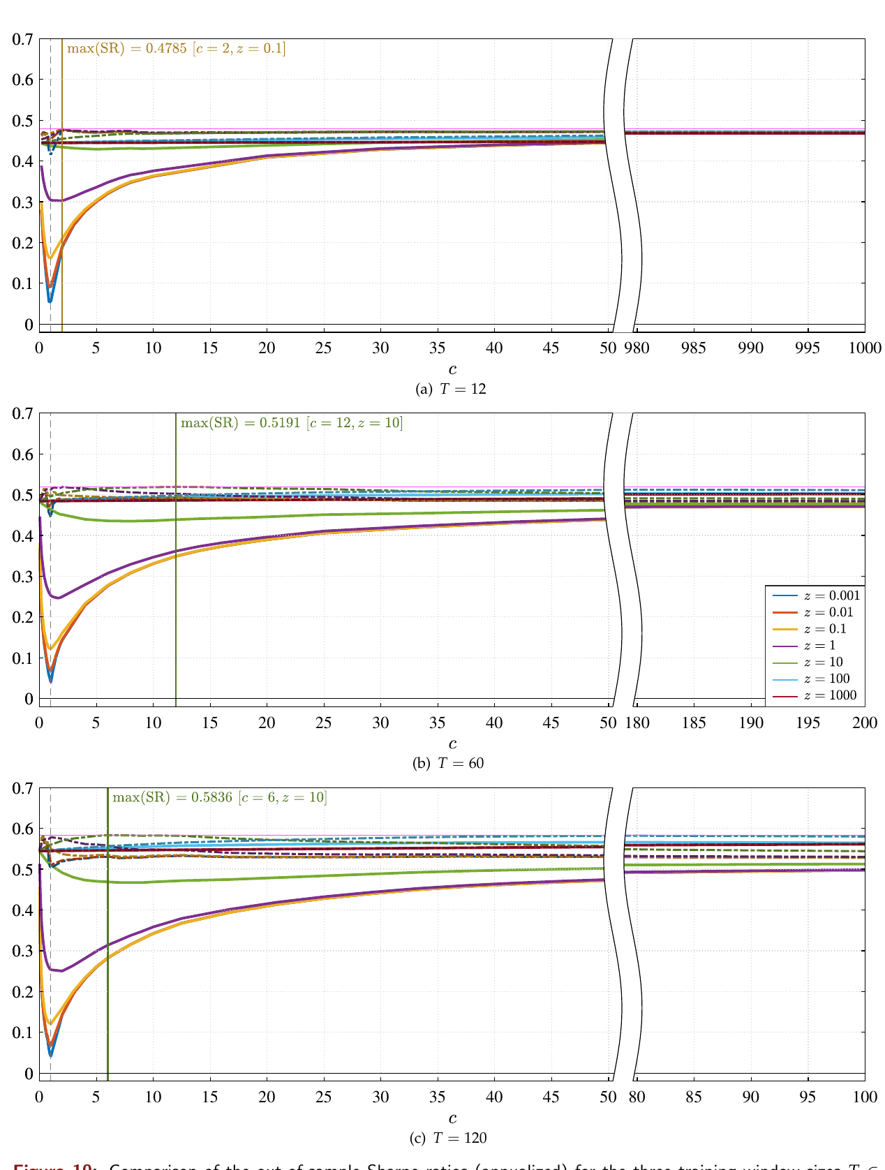
The figure is Buncic's comparison once the intercept is free. Solid lines average the Sharpe ratios of the 1,000 draws. Dash-dotted lines take the Sharpe ratio of the averaged forecast. The annotated peaks, 0.4785 at complexity 2, 0.5191 at complexity 12, and 0.5836 at complexity 6, are the maxima on Kelly, Malamud, and Zhou's seven penalty values. The finer grid that produced 0.5863 uses z of 2, which is not on that seven-point list, so it does not appear as a label. The shape is the same on both grids. The peak sits at low or moderate complexity. The far right of each panel, where c is largest, is flat and no higher. The 120-month panel sits above the 12-month panel. Belkin, Hsu, Ma, and Mandal's double-descent picture, which the factor-investing deck uses as the theoretical alibi for huge models, has test error falling again after the model passes the interpolation boundary at c of 1. There is a partial version of that dip and recovery in these panels. It tops out at complexity 2, 12, or 6, and then stops. It does not keep paying at complexity 1,000.
The long-only claim is the same restriction. With a zero intercept, a 12,000-feature model and a 500-feature model produce timing weights that look alike, and a heavily shrunk linear regression produces the same positivity. Free the intercept and the 12,000-feature weights correlate 0.9999 with a 100-feature model and 0.9661 with a regression on the long-term yield alone. The machine did not discover a sign restriction. The origin did.
Two cautions sit on these Sharpe ratios. They are the best of a wide penalty grid, picked on the same January 1940 to December 2020 window used to report them, with no deflation for the search. And month-t inflation, one of the 15 predictors, is not published until the middle of month t+1. Buncic lags it and the random-feature Sharpe ratios fall across the board. He does not print a single replacement number, so none is supplied here. None of the ratios deduct a spread. A monthly timing overlay on the market is cheap relative to a cross-sectional book. It is not free.
The bill is predictors over months
The question is why a short monthly sample cannot carry 12,000 coefficients. The variance piece of the prediction error grows in proportion to the number of coefficients divided by the number of months.
Shah's decomposition of expected squared error, his equation (1.5), splits the error of a fitted function into squared bias, variance of the fit, and the irreducible noise in the outcome. For ordinary least squares on d basis functions, the variance piece averages to his equation (3.1).
$$ \mathbb{E}\,R(\hat{h}_{D}) - \mathbb{E}\,R(\hat{h}_{X}) \approx \frac{\sigma^{2}\, d}{n} $$
Read it as an extra out-of-sample squared error, in the square of whatever units the outcome is in. Sigma-squared is the variance of the outcome given the predictors. d is the number of coefficients. n is the number of training observations. The old article "The Mathematics of Machine Learning, for Traders" derives the trace step. The usable fact is the ratio d over n.
Worked with the variance of R itself, 1.1985, as a stand-in for sigma-squared. That stand-in is reasonable here because these predictors explain little of next month, which is the whole equity-premium problem. Fifteen coefficients and 120 months: 1.1985 times 15 divided by 120 equals 0.150. Twelve thousand coefficients and 12 months: 1.1985 times 12,000 divided by 12 equals 1,198.5. The second bill is the complexity ratio, 1,000, times the noise variance. Ridge and the average across random draws are attempts to refuse that bill. They do not repeal the ratio. Buncic's bias numbers say the refusal failed on its own terms. For the 12,000-feature model, squared bias of the forecast sits between 0.0130 and 0.0267 when the intercept is forced to zero, and under 0.0002 once the intercept is free. The flexible model was the biased one.
The penalty you choose is a belief about how many of the predictors matter. Shah compares an ell-2 constraint, the ridge style, with an ell-1 constraint, the sparse style. Once each constraint is set to the smallest width that still contains the true coefficient vector, the excess-risk bounds are on the order of the square root of p over n for ell-2, and the square root of (s times the natural log of p) over n for ell-1, where s is the number of nonzero coefficients. Read the bounds as rates on excess prediction error. Smaller is a tighter guarantee.
Take p of 15, n of 120, and suppose s equals 2, which is an illustration, not a test result. Buncic's univariate horse race keeps surfacing the term spread and book-to-market, so two is a serious guess and still a guess. The ell-2 order is the square root of 15 divided by 120, which is 0.35. The ell-1 order is the square root of (2 times the natural log of 15) divided by 120, which is 0.21. If instead all 15 predictors matter, the ell-1 constraint has to open wide enough to hold a dense vector, and that order worsens to 0.58, while ell-2 stays at 0.35. A sparse penalty wins when you believe a few characteristics carry the premium. A ridge penalty wins when you believe the signal is spread out. That belief is the economic prior. It is an input. The fitting routine does not supply it.
Expected returns in Buncic's zero-intercept block make the same point in portfolio units. The 12,000-feature model, penalty 1,000, has annualized expected timing-strategy returns of 0.273, 0.079, and 0.044 at windows of 12, 60, and 120 months. The best expanding 15-predictor ridges have 0.571, 0.639, and 0.859. Divide 0.859 by 0.044 and you get 19.5. Buncic calls that close to twenty-fold. I am keeping his ratio and his wording. The table transcription in the source file is too garbled to re-read those cells off the grid, so the prose figures are the ones used here.
A network wants 24 countries; a regression does not
The question is whether a more flexible model ever earns its parameters. It does when the training set is a cross-section, and the extra return is 0.12 percentage points a month.
Chen, Hanauer, and Kalsbach run the comparison the equity-premium study cannot. One series gives you hundreds of months. A stock cross-section gives you a fresh panel every month. Their sample is 24 developed markets, 36 firm characteristics ranked each month within each country onto the interval from -1 to +1, microcaps removed (the smallest names making up 3 percent of country market cap), and value-weighted long-short quintiles. The test window is January 2002 to December 2021, 240 months. Training is an expanding window. The only lever is where the fit happens: a separate model for North America, Europe, Japan, and Asia Pacific, or one model on the pooled developed markets. The old article "Global vs Regional: When Complexity Wants More Data" keeps the screens and the hyperparameter grids. The numbers that decide the argument are in their Table 1.
Local ordinary least squares earns 0.47 percent a month (standard deviation 2.64, t-statistic 2.76). Global ordinary least squares earns 0.43 percent (standard deviation 2.76, t-statistic 2.44). The elastic net is the same pattern, 0.43 local against 0.39 global. Random forests tie at 0.52. Gradient-boosted trees go the other way, 0.51 local against 0.59 global (t-statistic 3.75). The neural-network ensemble goes further, 0.62 local (t-statistic 4.62) against 0.74 global (t-statistic 5.73). The crossover sits between the forest and the boosted trees. Linear models take a small local edge. The two flexible models take a global one.
Check the printed t-statistics against the printed means and standard deviations over 240 months. Ordinary least squares local: 0.47 divided by (2.64 over the square root of 240) equals 2.76, matching the print. Boosted trees global: 0.59 divided by (2.44 over the square root of 240) equals 3.75, matching the print. The global network: 0.74 divided by (1.99 over the square root of 240) equals 5.76, against their printed 5.73. The printed 5.73 stays. The gap fits a rounded standard deviation, or a robust standard error. The result does not move.
The 0.12 percentage-point gap, 0.74 minus 0.62, is 0.12 divided by 0.62, or 19 percent of the local network's own return. Their cumulative-performance figure prints 456 percent for the global network over the twenty-year test. Compounding the 0.74 percent mean for 240 months produces 487 percent. The figure is the compounded path, which sits under the compounded mean because volatile months do not compound at the average. 456 stays as the path.
Spanning regressions ask whether one book already contains the other. Regress the global network's long-short return on the local network's, and the intercept is 0.20 percent a month with a t-statistic of 3.45. Multiply 0.20 by 12 and you get 2.4 percent a year, an arithmetic scaling, not a compound. The boosted-tree version of that intercept is 0.15 percent a month, t-statistic 2.04. Run the regression the other way, local on global, and the network intercept is -0.07 with a t-statistic of -1.15. The local flexible model adds nothing once the global one is in the book. The linear models show no reliable intercept in either direction.
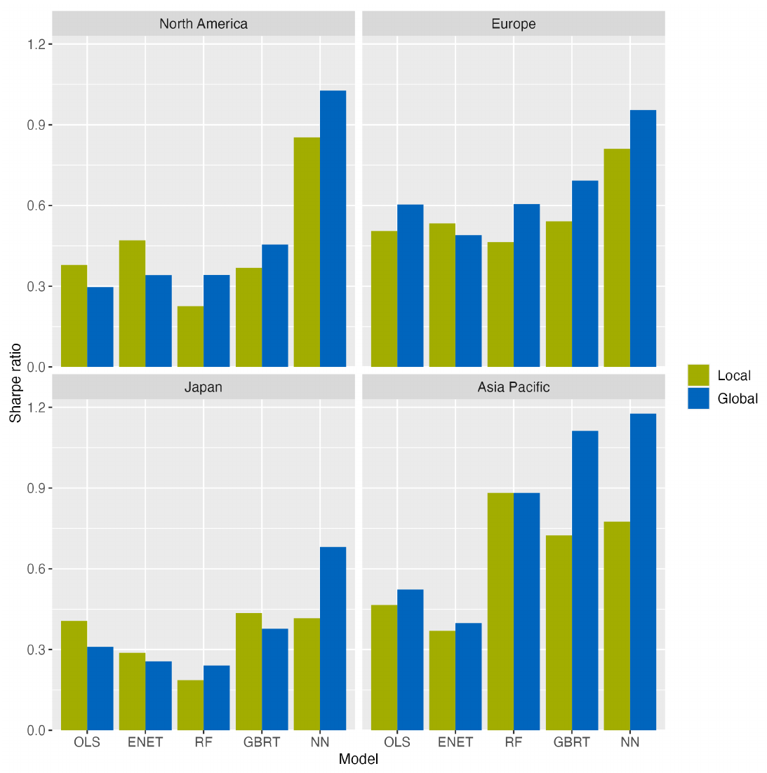
The regional Sharpe ratios, which the paper annualizes itself, repeat the split. The global network earns 1.03 in North America against 0.85 local, 0.96 against 0.81 in Europe, 0.68 against 0.42 in Japan, and 1.18 against 0.78 in Asia Pacific. Japan is the case the older linear literature treated as special, and the global network still leads there, by 0.68 minus 0.42, or 0.26. For ordinary least squares and the elastic net the paper reports a mixed pattern: global fits better in Europe and Asia Pacific, regional fits better in North America and Japan, and the gaps are small. The rank of characteristics onto [-1, +1], done inside each country, is already an economic prior. It is the cross-sectional rank, not the raw accounting ratio, that enters the fit. The network then needs the pooled sample to estimate the nonlinear pieces of that rank. The regression does not.
These Chen, Hanauer, and Kalsbach returns are gross. The paper does not report a cost cut. A monthly, value-weighted, country-neutral quintile book turns over less than a model that rebuilds every name's weight from scratch. How much less is not in the tables.
A fifth, then the turnover
The question is the size of the nonlinearity bonus a book should budget. The honest number in the factor-investing deck is about 20 percent on the Sharpe ratio, and the turnover attached to the published machine-learning books can erase it.
The deck prints two out-of-sample Sharpe ratios for each model. The first cut: a random forest at 2.19, a neural network at 3.21, a principal-components model at 3.21, and Kelly, Pruitt, and Su's instrumented principal-components model (IPCA) at 3.39. The second cut, with the first number repeated in parentheses: 0.86 (2.19), 2.39 (3.21), 2.77 (3.21), and 3.21 (3.39). These live on a different book from the 0.55 market-timing ratios above. They are cross-sectional factor portfolios, and the level is not comparable to a timing Sharpe on the market. The ranking inside the table is the usable fact. IPCA, a linear model that builds factors as combinations of characteristics, slips from 3.39 to 3.21. Divide 3.21 by 3.39 and subtract 1: a 5 percent slip. The neural network slips from 3.21 to 2.39. Divide 2.39 by 3.21 and subtract 1: a 25 percent slip. The most linear specification holds up. The old article "Does ML Actually Help Asset Pricing? Kelly's 20%, Not 2–3×" goes after the unfair part of the comparison, a three-factor baseline against a model fed hundreds of characteristics. Bryan Kelly's own sentence, as the deck records it, is the budget: a 20 percent increase in the Sharpe ratio from adding nonlinearities feels realistic, and a doubling does not.
Turnover is where that fifth goes to die. Avramov, Cheng, and Metzker measure monthly turnover of 0.976 on the Gu, Kelly, and Xiu machine-learning portfolio and 1.664 on a deep-learning stochastic-discount-factor portfolio. Size and value, in the same discussion, turn over below 10 percent a month. A book that replaces itself every month, or 1.66 times every month, pays the spread on the way in and on the way out. Avramov, Cheng, and Metzker also find the excess return concentrated in the short leg and in tiny, illiquid, distressed names, and they find the nonlinear models weaken once those names are dropped, while IPCA does not. A 20 percent Sharpe bump that lives in names you cannot short, at a turnover near 100 percent a month, is a research result. It is a poor order.
The rule at the desk
The question is what changes in the research process on Monday.
On a single monthly series, fit the mean, keep the predictor count near the Goyal-Welch 15, shrink with a small z, and use the long window. I am against replacing that ridge with 12,000 random features. The complex model lost to buy-and-hold, lost to a rolling historical average, and lost to the 15-predictor ridge with the intercept forced off and with it left on. The best random-feature specification, 0.5863, beats buy-and-hold by 0.5863 minus 0.5494, which is 0.037, and then loses to the ridge by 0.6990 minus 0.5863, which is 0.113. That 0.037 is the timing gain left behind by a flat refusal of every flexible model on this sample. It is smaller than the gain you give up by trading the headline model, and neither number has paid a spread or survived a penalty for searching the grid.
On a cross-section, add countries before adding layers. The network's global-minus-local gap is 0.12 percent a month, and the spanning intercept on the local network is 0.20 percent a month. Ordinary least squares does not want the pool: 0.47 local against 0.43 global. The prior that earns its place is the one you can say before the fit, a rank inside the country, a factor structure like IPCA, a penalty matched to how many characteristics you believe are real. Shah's rates are the reason. The ratio inside the variance bill is d over n. Grow n, from one market to 24, and a larger d becomes affordable. Leave n at 12 months and no penalty in the grid makes 12,000 features the right trade.
Budget a fifth on the Sharpe ratio for the nonlinear piece, then write down the turnover. If the book cannot pay a monthly turnover near 1, stay with the linear factor model that held 3.21 of its 3.39 in the deck's second cut. Complexity is a data-hungry regularizer with a modest payoff. The plot that called it a virtue was an intercept set to zero and an average of ratios.
KEY POINTS
- On one common window, January 1940 to December 2020, buy-and-hold earns a Sharpe ratio of 0.5494. The 12,000-feature model earns 0.4851. A 15-predictor expanding ridge with an intercept earns 0.6990. The best random-feature model, 200 features, penalty 2, 120 months, earns 0.5863.
- The rising complexity curve needs a zero intercept and a per-draw average of Sharpe ratios. Free the intercept and the best random-feature Sharpe rises with the window, from 0.4745 to 0.5157 to 0.5863. At 2 features and 120 months the per-draw average prints Sharpe ratios near -0.0017 next to positive expected returns.
- The variance bill is sigma-squared times coefficients over months. With the variance of the standardized excess return at 1.1985, 15 coefficients on 120 months cost about 0.15, and 12,000 coefficients on 12 months cost about 1,198. A sparse penalty tightens the bound only if few predictors matter.
- On 24 developed markets, the global neural network earns 0.74 percent a month (printed t-statistic 5.73) against 0.62 percent local. Ordinary least squares goes the other way, 0.47 local against 0.43 global. The global network's spanning intercept over the local network is 0.20 percent a month, t-statistic 3.45. Regional network Sharpes: 1.03, 0.96, 0.68, and 1.18 against local 0.85, 0.81, 0.42, and 0.78.
- Budget about 20 percent on the Sharpe ratio for nonlinearities. In the deck's two cuts, linear IPCA slips from 3.39 to 3.21 and the neural network slips from 3.21 to 2.39. Monthly turnover on the published machine-learning books is 0.976 and 1.664, against under 10 percent for size and value.
- The 0.6990 and 0.5863 are maxima over a penalty grid, scored on the window used to pick them. Inflation in the predictor set prints two weeks late. No Sharpe ratio above has paid a spread. The global-network t-statistic implied by the printed mean and standard deviation is 5.76, against the printed 5.73. Buncic's mean, standard error, and t-statistic for the standardized return do not multiply through.
References
- The Virtue of Complexity in Return Prediction (Kelly, Malamud, Zhou, 2024)
- Comment on 'The Virtue of Complexity in Return Prediction' (Berk, 2023)
- Simplified: A Closer Look at the Virtue of Complexity in Return Prediction (Buncic, 2025)
- Model Complexity and the Performance of Global versus Regional Models (Chen, Hanauer, Kalsbach, 2025)
- Mathematics of Machine Learning (Shah)
- Machine Learning in Factor Investing (DDA3600)