3. Robust Systems Lab October 5, 2026 18 min

3.43 Building a Statistically Valid Backtest: The Checklist Nobody Runs

Backtest overfitting: stock predictors fall 26% out of sample and 58% after publication, and the median Sharpe of 215 smart-beta strategies falls 73% once live.

McLean and Pontiff record stock-portfolio predictors whose performance is 26% lower out of sample than in sample, and 58% lower after publication. Suhonen, Lennkh, and Perez look at 215 smart-beta strategies banks offered and find a median deterioration of 73% in the Sharpe ratio from the backtest to the live period. Arakelian, Bolesta, Liu, Osterrieder, Poti, Schwendner, Sutiene, Vlah Jerić, and Weinberg take those two results as the case for a valid backtest. The machinery they assemble is the probability of backtest overfitting, White's reality check, Hansen's test of superior predictive ability, and Romano and Wolf's stepwise test. Underneath sit an out-of-sample split you do not retune, a cost, a size cap, and a permutation against chance. A Sharpe ratio that has not been through that machinery is a sales exhibit.

What this actually is

You have a monthly equity factor, or an ES rule, with an in-sample Sharpe ratio of 1.4 across ten years. You tried 40 variants. The memo holds the winner. The other 39 stay off the page. The 1.4 is the maximum of that search, and the maximum of a noisy search sits above the noise.

The method scores how often a selection of that kind places the in-sample winner below the median on data the rule never saw. It also tests whether any rule beat a benchmark you named in advance, with the full set of rules as the hypothesis.

A youth-league tryout runs the same way. Forty kids shoot free throws for an hour. You take the kid with the most makes. The next session that kid looks ordinary, because the hour mixed skill with luck and you kept the luck. A bigger tryout produces a higher score on the day and a worse next session.

Ship under that claim and you freeze the rule before the holdout year, subtract slippage and commission before you quote a profit factor, cap leverage at the size the margin desk will fund, and replace the winner's t-statistic with a test of the whole set. Trust a backtest that skips those steps and the live Sharpe ratio is the one Suhonen, Lennkh, and Perez measured, a median 73% below the tear sheet, on 215 products a bank was willing to sell. Apply the same steps to a real edge that is too small to clear a multiple-testing bar and you stay with the benchmark. Staying with the benchmark is the cheaper mistake.

The in-sample winner finishes below the median

The question is whether the strategy you would have picked in sample still sits in the top half once the sample changes.

Bailey, Borwein, Lopez de Prado, and Zhu supply the definition, and the discussion paper reprints it. There are N strategies. Rank each one from 1 to N on the in-sample performance measure, with N the best rank and 1 the worst, and rank them again on the out-of-sample measure. The selection overfits when the expected out-of-sample rank of the in-sample winner is at or below N/2.

$$ \sum_{n=1}^{N} E\left[\bar{r}_{n} \mid r \in \Omega_{n}^{*}\right] \operatorname{Prob}\left[r \in \Omega_{n}^{*}\right] \leq \frac{N}{2} $$

Read it as: N is a count of strategies. r is the in-sample rank vector and r-bar is the out-of-sample rank vector, both in rank units from 1 to N. Omega-star sub n is the set of rankings in which strategy n is the in-sample winner, meaning its in-sample rank equals N. The probability in front is the chance that n wins the in-sample horse race. The term inside the expectation is n's out-of-sample rank on those occasions. The sum is one number, the expected out-of-sample rank of whoever won in sample. The process overfits when that number is at or below N/2.

The probability of backtest overfitting, PBO, is the chance that this winner's out-of-sample rank falls below that same cutoff.

$$ \mathrm{PBO} = \sum_{n=1}^{N} \operatorname{Prob}\left[\bar{r}_{n} < \frac{N}{2} \mid r \in \Omega_{n}^{*}\right] \operatorname{Prob}\left[r \in \Omega_{n}^{*}\right] $$

Read it as: PBO is a probability between 0 and 1, with no market unit. For each strategy n, take the probability that its out-of-sample rank is below N/2 given that it won in sample, multiply by the probability that it won, and add the N products. The discussion paper prints a strict inequality. Rank equal to N/2 does not count as a miss.

The ten splits below are constructed so both sums can be checked by hand. They are not a price series. N is 5, so N/2 is 2.5. Ranks 1 and 2 are misses. Rank 3 is not. The paper calls N/2 the median of the ranks. For five strategies the middle rank is 3, and the formula's cutoff is 2.5. The arithmetic below uses 2.5, the number in the formula. With an even count the printed cutoff is harsher than a bottom half: four strategies give N/2 equal to 2, and the strict inequality keeps only rank 1.

Split	In-sample winner	Out-of-sample rank
1	A	1
2	A	2
3	B	4
4	C	1
5	A	2
6	D	2
7	B	5
8	C	1
9	E	4
10	A	2

The out-of-sample ranks of the in-sample winner are 1, 2, 4, 1, 2, 2, 5, 1, 4, 2. Seven of the ten sit below 2.5, so the miss rate is 7/10, which is 0.70. The weighted sum matches. A wins 4 of 10 splits and misses all 4, contribution 0.40 times 1. B wins 2 and misses none, contribution 0. C wins 2 and misses both, contribution 0.20. D wins 1 and misses it, contribution 0.10. E wins 1 and finishes at rank 4, contribution 0. 0.40 plus 0.20 plus 0.10 equals 0.70.

The expected out-of-sample rank uses the same weights. A's mean rank on its four wins is (1 + 2 + 2 + 2) / 4 = 1.75. B's is (4 + 5) / 2 = 4.5. C's is 1. D's is 2. E's is 4. Then 1.75 times 0.40, plus 4.5 times 0.20, plus 1 times 0.20, plus 2 times 0.10, plus 4 times 0.10, equals 0.70 + 0.90 + 0.20 + 0.20 + 0.40 = 2.40. The plain average of the ten ranks is 24/10 = 2.4. The two routes agree. Because 2.4 is below 2.5, the paper's definition calls this selection overfit. The comparison for the 0.70 is a uniform out-of-sample rank, the case where the in-sample win carries no information about the out-of-sample rank. Each of the five ranks then has probability 1/5, and only ranks 1 and 2 sit below 2.5, so the miss probability is 2/5 = 0.40. The expected rank is (1 + 2 + 3 + 4 + 5) / 5 = 3, which sits above the cutoff of 2.5, so a uniform rank does not meet the overfitting definition. The toy's 0.70 against that 0.40, and its 2.4 against that 3, are the gap the definition is built to catch.

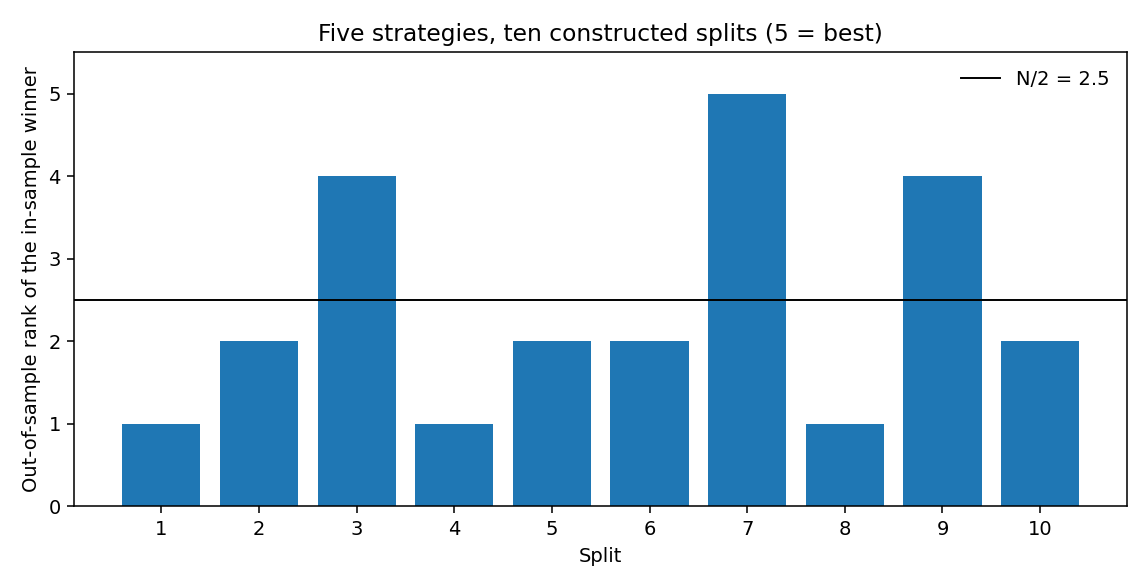
Out-of-sample rank of the in-sample winner on ten constructed splits of five strategies. Seven of the ten ranks sit below the line at 2.5

The discussion paper stops at the definition. It does not compute a PBO on a price series, so 0.70 is not a market result. The number you would take to a committee comes from reshuffling which slice of your own sample is the training slice and recording where the training winner finishes on the held-out slice. Bailey, Borwein, Lopez de Prado, and Zhu estimate that probability with combinatorially symmetric cross-validation. The discussion paper names the probability and does not show the reshuffle. The old article "The Backtest Integrity Checklist" is where that reshuffle becomes a line you either pass or you do not ship.

White's reality check tests the whole search

The question is whether any model beat a benchmark, once the hypothesis is the entire search and not the winner you noticed.

White's reality check starts from a loss. For each model k and each date, form the loss of the benchmark minus the loss of model k. A positive gap means model k lost less than the benchmark on that date.

$$ \delta_{k,t} = L\left(y_{t+h},\hat{y}_{t+h,\mathrm{BM}}\right) - L\left(y_{t+h},\hat{y}_{t+h,k}\right) $$

Read it as: delta sub k,t is the loss gap for model k at date t, in whatever unit the loss uses. y at t plus h is the outcome h steps ahead. The two y-hats are the benchmark forecast and model k's forecast of that outcome, both formed with information dated t. L is the loss. The paragraph above this equation in the discussion paper writes the forecast with a lag, time t minus h. The equation writes t plus h, which is the timing in White: you score a forecast of the outcome h steps ahead. The equation is the one used here.

The null says the best model has no positive expected gap.

$$ H_{0}: \mu = \max_{k=1,\ldots,m} E(\delta_{k}) \leq 0 $$

Read it as: m is the count of models. E(delta sub k) is model k's expected loss gap, in loss units per date. Mu is the largest of those m expectations. The null says mu is zero or negative, so no model beats the benchmark on average. The alternative says mu is positive, so at least one does. The sentence beside this display in the discussion paper does not match it. That sentence says the null compares loss differentials to benchmark losses, and then says model losses are larger than the benchmark. Use the display.

Take the loss to be the negative of the monthly return, in percentage points. Then delta equals the model's return minus the benchmark's return, and the units stay in percentage points per month. Four months, three models, built so the arithmetic is checkable. This is not a price history.

The benchmark returns 1, 1, 2, 0. Model 1 returns 3, 1, 3, 1, so its gaps are 2, 0, 1, 1. Model 2 returns 4, 0, 2, 2, so its gaps are 3, minus 1, 0, 2. Model 3 returns minus 1, 2, 2, minus 1, so its gaps are minus 2, 1, 0, minus 1. The means are 1, 1, and minus 0.5 percentage points per month. The maximum is 1, shared by model 1 and model 2. Check model 1 through the loss rather than the return shortcut: benchmark losses are minus 1, minus 1, minus 2, 0, and model 1's losses are minus 3, minus 1, minus 3, minus 1. Subtracting gives 2, 0, 1, 1. Same gaps.

Model 1's gaps deviate from 1 by +1, minus 1, 0, 0. The sum of squares is 2. Divide by 3, one less than the four months, and the sample variance is 2/3. The standard error is the square root of that variance, divided by the square root of 4. The t-statistic is the mean gap divided by that standard error, a unit-free measure of how far the mean sits from zero given the scatter across months. For model 1 it equals the square root of 6, which is 2.45. Model 2 has the same mean of 1 and a sum of squared deviations of 10, and the same steps give a t-statistic of 1.10. The path is wider, from +3 to minus 1, so the same average edge is a weaker statistic. Model 3's mean is minus 0.5 and its sum of squared deviations is 5, and the t-statistic is minus 0.77.

The one-sided p-value on model 1 alone, one-sided because the alternative is a positive gap, with 3 degrees of freedom left after estimating the mean, is 0.046. The one-sided 5% critical value of that t distribution is 2.35, and 2.45 sits above it. That p-value belongs to a single model. The search had three. The discussion paper points at the Bonferroni bound as one way to cap the p-value of a multiple test. The bound splits one 5% budget for the whole search by the model count, so that a false pass anywhere in the set stays inside that budget. Here 0.05 divided by 3 is 0.0167, and the critical t-statistic on 3 degrees of freedom rises from 2.35 to 3.74. Model 1's 2.45 misses 3.74.

White's reality check replaces that bound with the joint distribution of the models. Bonferroni treats the models as separate. Models scored on the same four months share the months, so their gaps move together, and the null distribution of the maximum is tighter than the Bonferroni corner. The discussion paper says an analytic form for that distribution is not practical. You resample the dates, recompute the maximum on each resample, and read the p-value from the resampled maxima. Four months will not support a resample you should trust, because a draw can repeat one month until the standard deviation collapses. No bootstrap p-value is printed here for that reason. The object of the test is still the maximum, and the crude bound the paper cites sits above the best t-statistic in the toy.

The paper says the procedure holds the family-wise error rate, the probability of one or more false discoveries, at a preset level alpha. Alpha is the false-rejection rate you pick before seeing the models. A common choice is 0.05. One sentence then gets the error backwards. It says the procedure caps the chance of a wrong rejection when the null is false. A rejection of a false null is the correct decision. The cap applies when the null is true: no model beats the benchmark, and the test says one does. The formulas earlier in the section match that second statement.

Hansen's test of superior predictive ability is a repair for a different defect. White's null is built under the least favorable configuration, the case in which every model, including model 3 with a mean gap of minus 0.5, is treated as if its expected gap were zero. A hopeless model can still win the maximum by luck, the critical value rises, and a real model fails the test. Stack more poor models into the race and that critical value rises further. Hansen recenters so that a model which is inferior by a clear margin does not enter the null as a tie with the benchmark. The discussion paper also calls this a test of superior predictive performance. The 2005 title is superior predictive ability. Hansen's answer is whether any model is superior. The names of those models are a separate step.

Romano and Wolf walk the list. Rank the models by the statistic. Test the best one against a critical value computed from the whole set. If it fails, stop, and the set of superior models is empty. If it passes, drop it, recompute the critical value on what remains, and continue until a model fails. On this toy the best statistic is model 1's 2.45. That sits above the single-test critical value of 2.35, and the Bonferroni bound on the same three models is 3.74. The stepwise critical value is a resampled quantile. Four months will not support that resample, so the bound you can compute by hand is the Bonferroni one, and model 1 misses it. The illustrated output is an empty set.

A later paragraph in the discussion paper calls the Romano and Wolf procedure a false-discovery-rate method. The 2005 paper controls the family-wise error rate, the chance of any false inclusion. So does the discussion paper's own account of the stepwise test, earlier in the same section. The false discovery rate would cap the share of rejected models that are false, and it would let more models through. The name in the later paragraph is a different test. A quadratic form in all the forecast errors at once is the other route the paper considers, and it needs a covariance matrix that is close to singular when the model count is large, so the chi-squared limit does not arrive. That is why these tests bootstrap a maximum t-statistic. The paper says the bootstrap is heavy enough that machine-learning backtests in production often skip it. Skip it and the number you are left holding is the single-model p-value of 0.046.

Hold out, charge the cost, cap the size, permute

The question is which operating rules keep the backtest in the same units as the account.

The out-of-sample split comes first. The discussion paper's schematic puts portfolio weights, the holding period, and the rebalancing dates inside a train window, then a split point, then a test window. The drawing is the easy part. The rule is the sentence beside the overfitting definition: once you change the model so that it also looks good on the test window, that window is in sample. One retune after you have seen the holdout, and the split no longer separates anything. A longer test window estimates the performance with less noise. The window has to stay untouched, including by the person who picks the variant to report.

Costs come next. Profit factor is the sum of winning trades divided by the sum of absolute losing trades, a ratio with no unit. Ten trades, wins of 5, 4, 3, 2, and 1 percentage points, absolute losses of 1, 1, 2, 2, and 3. The profit factor is 15/9, which is 1.67. Charge 50 basis points of slippage and commission on each trade. A basis point is 0.01 of a percentage point, so the charge is 0.5 percentage points, subtracted from each win and added to each absolute loss. The wins become 4.5, 3.5, 2.5, 1.5, and 0.5, summing to 12.5. The absolute losses become 1.5, 1.5, 2.5, 2.5, and 3.5, summing to 11.5. The profit factor is 12.5/11.5, which is 1.09. The paper's instruction is to deduct that charge on every simulated trade and recompute the profit factor, the expectancy, and the drawdown. The gap between 1.67 and 1.09 is where a high-turnover rule loses the edge the gross number advertised. The paper does not choose the 50 basis points. You take the charge from the asset, the venue, and the size you intend to trade. A charge of zero is how the backtest overstates the live result.

Size after that. An edge of 2% a year on notional, with a volatility of 15% a year, is a Sharpe ratio of 2/15, which is 0.13. Both the return and the volatility are fractions of notional per year, so the ratio has no unit. At ten times leverage the account shows a 20% return and a 150% volatility, and 0.20 divided by 1.50 is still 0.13. A year one standard deviation below the mean is 0.20 minus 1.50, a loss of 130% of equity. The tear sheet printed the 20%. The edge was 2%. Full leverage, a position in every name, and no size cap inflate the profit and ignore margin, liquidity, and a drawdown limit. Scale the simulated trades to a maximum the account can hold, then recompute the same ratios.

The permutation is the comparison to chance. The paper wants the strategy's result set against a null of random hypothetical strategies, by Monte Carlo, with the costs left on. A profit factor of 1.09 that sits in the middle of that null is luck. The same comparison shows up inside the reality check as a resampling of the dates. Either way you compare the result to the distribution of random rules that have no edge. The old article "Replication Notebook Template: Claim → Replicate → Stress → Verdict" puts this comparison in the stress beat. Run it on the rule you froze before the holdout, on the same cost and the same size cap.

Two further items from the paper's list, both easy to game. Sensitivity moves the entry, the size, and the indicator across a range you would have accepted before the search, and asks whether the profit factor stays above 1. A profit that exists at one setting and vanishes next door is a fit to the path. Walk-forward rolls the train window, re-estimates, and stitches the test periods. A single calm decade is a weak test, which is the paper's point. Choosing the window length from the stitched result puts those test periods back into the search.

The survey that precedes the list names the area under a ROC curve, a Kolmogorov-Smirnov comparison, information value, and a Hosmer-Lemeshow grouping. Those four score a predicted probability against an outcome, which is the job of a default model. A trading rule's result is a return after cost. Leave them off this checklist.

The paper's closing recommendations are thinner than the list: hold out data and keep it clean of snooping, score stability and complexity rather than mean squared error alone, train the people who run the tests, and talk to outside researchers. The four that change a number on a tear sheet are the untouched holdout, the cost, the size cap, and the permutation. The old article "The Backtest Integrity Checklist" turns those into pass-fail lines. This paper is the argument for having the lines.

The haircut the citations report

The question is how large a haircut the papers in the reference list put on a raw in-sample result.

McLean and Pontiff, on predictors of the cross-section of stock returns: performance 26% lower out of sample than in sample, and 58% lower after publication. Index the in-sample figure at 100. Subtract 26 and the out-of-sample index is 74. Subtract 58 and the post-publication index is 42. Those two complements are arithmetic from the declines the discussion paper quotes, not extra statistics. Falck, Rej, and Thesmar record a 50% decline in the performance of systematic strategies after publication, so the same style of index sits at 50. Suhonen, Lennkh, and Perez, on the 215 smart-beta strategies: the median Sharpe ratio deteriorates 73% from the backtest to the live period, so a backtest Sharpe ratio indexed at 100 sits at 27 live. The four bars come from three measurements, a return, a performance decline, and a Sharpe ratio. All four point down.

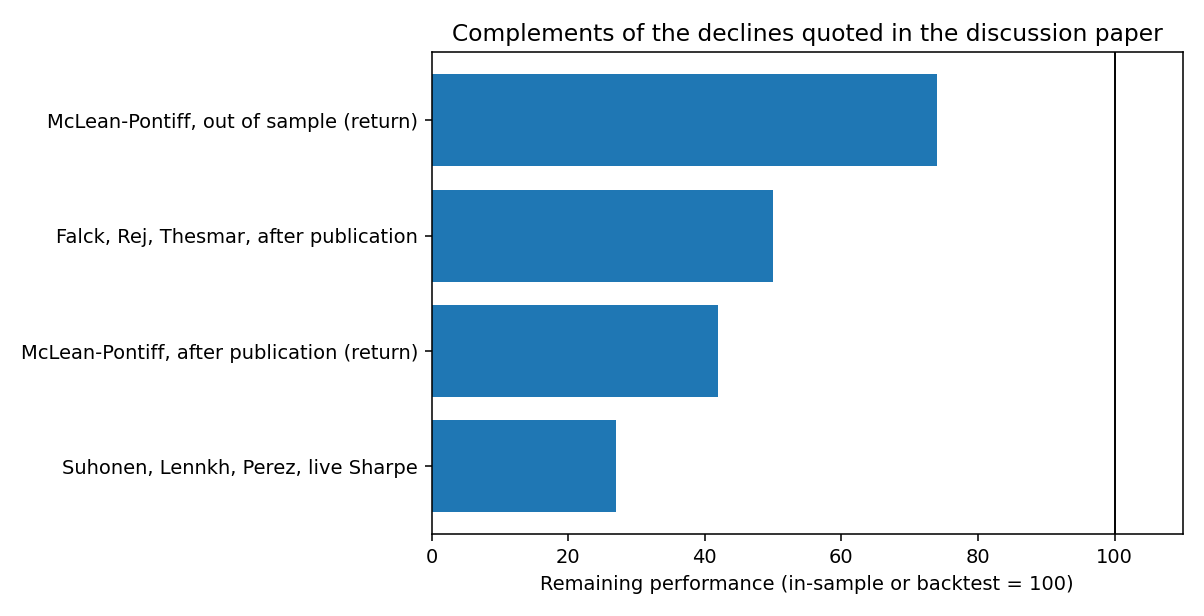
Remaining performance after the declines quoted in the discussion paper. In-sample or backtest is 100. McLean and Pontiff: 74 out of sample and 42 after publication. Falck, Rej, and Thesmar: 50 after publication. Suhonen, Lennkh, and Perez: 27 on the live Sharpe ratio

Jensen, Kelly, and Pedersen reach the other conclusion. The discussion paper says they find a high degree of validity for factor strategies after publication, in the United States and abroad. It prints no magnitude for that finding, so they are absent from the chart. The discussion paper does not adjudicate the disagreement. A reader should not adjudicate it from this paper either. There is no new backtest in it. The MACD exhibits are terminal screens of an S&P 500 moving-average convergence rule, with buy marks, sell marks, and a block of descriptive trade counts. Change the sample or the bar size and the picture changes, which is the observation the screens are there to support. Descriptive counts are not a reality check.

Wiecki, Campbell, Lent, and Stauth are cited for the statement that backtests overstate live performance, with no magnitude attached in this discussion. The magnitudes the discussion paper does print are McLean and Pontiff's 26% and 58%, Falck, Rej, and Thesmar's 50%, and the 73% median Sharpe-ratio deterioration on the 215 live products.

Use those as a prior while your own reality check is still unrun. Take 26% off an in-sample return on the way to a fresh sample, and 58% off after publication. Take 73% off a marketed smart-beta Sharpe ratio on the way from the tear sheet to the account. That prior is a set of cited declines, and Jensen, Kelly, and Pedersen are the reminder that a factor with a reason can survive the publication date. You measure survival on a holdout you did not retune.

KEY POINTS

McLean and Pontiff's stock-portfolio predictors run 26% lower out of sample than in sample, and 58% lower after publication. On 215 smart-beta strategies that banks offered, Suhonen, Lennkh, and Perez find a median Sharpe-ratio deterioration of 73% from backtest to live. Falck, Rej, and Thesmar record a 50% decline after publication. Indexed to 100, the complements are 74, 42, 27, and 50.
The probability of backtest overfitting is the chance the in-sample winner finishes with out-of-sample rank below N/2. On a constructed set of five strategies and ten splits, 7 of 10 winners finish below 2.5, the weighted sum equals 0.70, and the expected out-of-sample rank is 2.4, which meets the paper's overfitting cutoff of 2.5. The 0.70 is a worked sum, not a market estimate. The discussion paper does not compute a PBO on prices.
White's reality check tests the best loss gap in the whole search. With loss equal to minus the return, three toy models over four months post mean gaps of 1, 1, and minus 0.5 percentage points. The t-statistics are 2.45, 1.10, and minus 0.77. The single-model one-sided p-value of 0.046 dies under the Bonferroni bound the paper cites: critical t rises from 2.35 to 3.74.
Hansen's superior predictive ability test stops treating hopeless models as ties with the benchmark, which is what makes White's null conservative. Romano and Wolf's 2005 stepwise test then names which models survive, controlling the family-wise error rate. A later sentence in the discussion paper calls that procedure a false-discovery-rate method. That name is the wrong test. Another sentence caps rejections "when the null is false," which reverses a type I error. Follow the formulas.
Before a number leaves the building: an untouched holdout, a cost taken off every trade (the toy profit factor falls from 15/9 = 1.67 to 12.5/11.5 = 1.09 at 50 basis points), a size cap (2% on notional at 15% volatility is a Sharpe ratio of 0.13, and 10x leverage still has Sharpe 0.13 while a one-sigma year loses 130% of equity), and a permutation against random rules. ROC curves and Hosmer-Lemeshow tests score default probabilities. They do not score this.
Jensen, Kelly, and Pedersen are the dissent the discussion paper reports and does not settle: factor strategies can stay valid after publication. This paper runs no new backtest. The haircut above is a prior, and the measurement is your own holdout.