6.59 Polynomial Regression Bands With a Profit Factor Below One
Nasdaq-100 polynomial regression bands: the four-degree model is crowned on a 0.55 profit factor. That 0.55 is one losing stock, and average profit factor falls from 1.76 to 1.60.
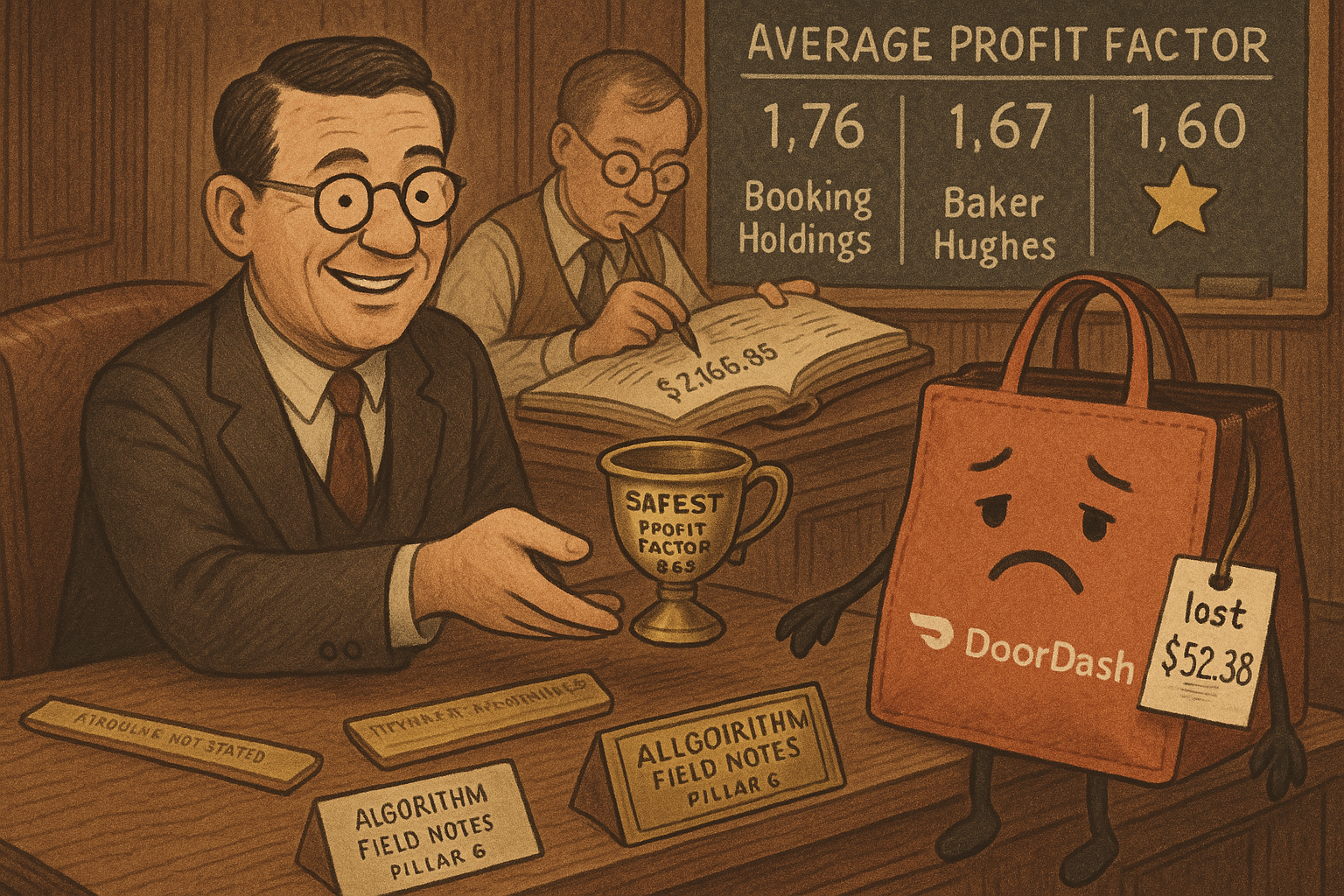
Gil Cohen fits second-, third-, and fourth-degree polynomial moving regression bands to Nasdaq-100 names from 2017 through March 2024, charges 0.3% on each fill, and names the four-degree model best. Table 3 puts the average net profit at 162.75 dollars per name. The abstract, the conclusion, and Table 4 print 162.73. The risk case next to that crown is a profit factor of 0.55 and a minimum win rate of 41.51%. Profit factor is gross profit divided by gross loss. At 0.55 the gross loss is 1.82 dollars for each dollar of gross profit.
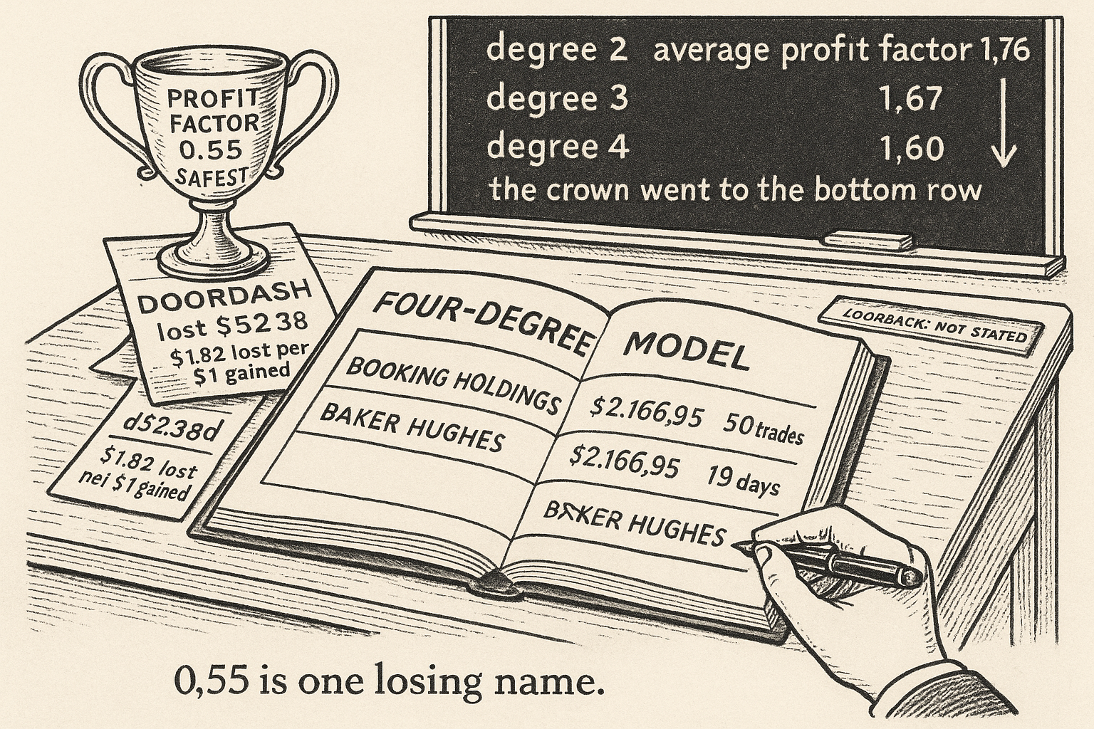
That 0.55 is DoorDash. It is the smallest profit factor in the four-degree column, on a name that lost 52.38 dollars. The average of the hundred profit factors is 1.60, down from 1.76 at degree 2 and 1.67 at degree 3. The model called the safe one has the worst average profit factor of the three.
What this actually is
You run Nasdaq-100 names, or you are about to let a script run them, and the offer is a band system with a seven-year daily backtest. The window is 2017 through March 2024, one hundred tickers, fills at the next open, and a commission of 0.3% on the buy and 0.3% on the sell. He says the printed results include those commissions. The curve he wants you to trade is a four-degree polynomial. The safety figure attached to it is a profit factor of 0.55, with a minimum win rate of 41.51% beside it.
The system fits a polynomial of price on a time index, draws a band two residual standard deviations above the curve and two below it, buys the next open after the close has crossed the upper band, and sells the next open after the close has crossed the lower band. The book is long or flat.
A flexible ruler on a paper chart is the same object. Allow one bend and the chalk line follows the broad swing. Allow two further bends and the chalk line ducks with the smaller turns, and the lane moves with it. You buy a step outside the lane on the way up. You sell a step outside the lane on the way down.
Take the ranking as a portfolio result and you trade degree 4, and you size as if 0.55 were the strategy's loss ratio. The bill for that reading is specific. The 0.55 is one losing name. The average profit factor is lower at degree 4 than at degree 2. The dollar average that won the horse race is fattened by a four-digit stock printed a second time under another ticker. The lookback, the number of days the ruler is pressed onto, is not in the paper.
The close sends the order
The order is a close through a band, filled at the next open. Degree changes the curve the bands hang on. The order stays that close.
$$ Y = \beta_0 + \beta_1 X + \beta_2 X^{2} \pm 2S $$ $$ Y = \beta_0 + \beta_1 X + \beta_2 X^{2} + \beta_3 X^{3} \pm 2S $$ $$ Y = \beta_0 + \beta_1 X + \beta_2 X^{2} + \beta_3 X^{3} + \beta_4 X^{4} \pm 2S $$
Read it as three fitted prices, in dollars per share. Y is the band, not a forecast he then scores on its own. X is a time index. Beta zero is the intercept in dollars. Each further beta multiplies a power of X, so the units of beta have to cancel that power back into dollars. S is the residual standard deviation in dollars, and the bands sit two of those above and below the curve. The first line is degree 2, the second degree 3, the third degree 4. He publishes no betas, no S, and no length for X. The numbers below are an illustration of the arithmetic, with coefficients chosen here so the powers stay easy to check. They are not his fit.
Set beta zero to 10 dollars, beta one to 0.5 dollars per day, beta two to 0.02 dollars per day squared, and S to 1.5 dollars. At day 10 the degree-2 curve is 10 plus 0.5 times 10 plus 0.02 times 100, which is 10 plus 5 plus 2, so 17 dollars. Two residual standard deviations are 3 dollars. The upper band is 20 and the lower band is 14. A close at 20.50 sends a buy for the next open. A later close at 13.50 sends the sell.
Add a degree-4 pair, beta three at 0.001 and beta four at minus 0.0001. At day 10 those terms are 0.001 times 1,000 and minus 0.0001 times 10,000, which is plus 1 and minus 1. The curve is still 17 dollars, and the bands do not move. At day 20 the degree-2 curve is 10 plus 0.5 times 20 plus 0.02 times 400, which is 28 dollars, and its upper band is 31. The degree-4 curve is 28 plus 0.001 times 8,000 minus 0.0001 times 160,000, which is 28 plus 8 minus 16, so 20 dollars, and its upper band is 23. A close at 24 is a buy on degree 4 and a nonevent on degree 2. Same closes, different orders, eight dollars of curve from two extra powers. On a short window those extra powers fit noise. On a long window the extra powers add a small bend. The paper does not state the window.
The 0.55 is DoorDash, and DoorDash lost money
The profit factor in the abstract is one cell, and the identity that turns it back into dollars is fixed by his own definitions.
$$ PF = \frac{GP}{GL} $$ $$ GL = \frac{NP}{PF - 1}, \qquad GP = PF \times GL $$
Read it as two steps, both in dollars except the ratio. PF is the profit factor, a pure number. GP is the gross profit, the sum of the winning trades, in dollars. GL is the gross loss, the sum of the losing trades written as a positive number of dollars. NP is net profit in dollars, and under those definitions it equals GP minus GL. Substitute GP equals PF times GL and you get NP equals GL times (PF minus 1), which rearranges to the second line. When the name made money, PF is above 1 and NP is positive. When the name lost money, PF is below 1 and NP is negative, so the ratio of two negatives is a positive gross loss. A profit factor of 1 means the gross profit equals the gross loss and the net profit is zero.
DoorDash, degree 4: net profit minus 52.38 dollars, profit factor 0.55, win rate 42.86%, 21 closed trades, 19 days in the average trade. Gross loss is minus 52.38 divided by (0.55 minus 1), which is minus 52.38 divided by minus 0.45, so 116.40 dollars. Gross profit is 0.55 times 116.40, so 64.02 dollars. Check: 64.02 minus 116.40 is minus 52.38, and 64.02 divided by 116.40 is 0.55. Divide 116.40 by 64.02 and the loss ratio is 1.818, which is 1 over 0.55. DoorDash paid 1.82 dollars of gross loss for each dollar of gross profit. That is the number offered as evidence the four-degree strategy is less risky.
The same inversion on a winner has to clear the other sign. Apple, degree 4: net profit 72.35 dollars, profit factor 1.70. Gross loss is 72.35 divided by 0.70, so 103.357 dollars. Gross profit is 1.70 times 103.357, so 175.707 dollars. The difference is 72.35 and the ratio is 1.70. The identity holds on a profit and on a loss.
Three different names own the three "minimum" headlines in Table 4. PDD Holdings owns the minimum net profit, minus 95.52 dollars, with a profit factor of 0.59 and a win rate of 51.28%. A name that wins half its trades and still prints a profit factor of 0.59 lost money because the losers were larger than the winners. Walgreens owns the minimum win rate, 41.51%, with a profit factor of 0.77 and a net profit of minus 20.07 dollars. DoorDash owns the minimum profit factor, 0.55. The conclusion then calls minus 95.52 "the lowest average loss" and prints it as 95.52 dollars, without the minus. The average net profit on that model is positive 162.75 dollars. The minus 95.52 is one name's net profit, the worst one, and the sign is the result.
Thirteen names in the four-degree table have a profit factor below 1. Twelve do in the three-degree table. Twenty do in the two-degree table. The prose for the two-degree model says 19 names lost money, and 19%. The column contains 20 negative net profits, including CSGP at minus 0.86 dollars. Keep his sentence, and treat the count as a possible miscount. The source and the column disagree.
Average dollars rise, and the average profit factor falls
The horse race he publishes is an average of dollars. The profit factor he also publishes, the average of the hundred ratios, goes the other way.
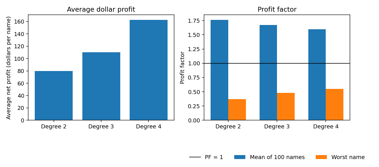
Degree 2: average net profit 79.67 dollars, average win rate 52.89%, average profit factor 1.76, worst profit factor 0.37 (Walgreens). Degree 3: 110.33 dollars, 55.85%, 1.67, worst profit factor 0.48 (Walgreens again). Degree 4: 162.75 dollars, 55.45%, 1.60, worst profit factor 0.55 (DoorDash). Win rate peaks at degree 3, not at degree 4. The floor he advertises does rise, from 0.37 to 0.48 to 0.55, and every one of those floors is a losing name. A higher floor under 1 is a smaller loss on the worst ticker. It is a loss.
Sum the reconstructed gross profits and gross losses across names and you get a different profit factor, the one a single dollar pile would have. Degree 2: gross profit 26,122.01 dollars, gross loss 18,154.68, ratio 1.44. Degree 3: 31,542.25 over 20,508.81, ratio 1.54. Degree 4: 40,302.88 over 24,027.84, ratio 1.68. Drop the cloned Baker Hughes row and the four-degree ratio is 36,542.58 over 22,434.49, which is 1.63. The dollar-weighted ratio rises with degree. The average of the ratios falls. He ranked on the average of the dollars, then described the risk with the minimum ratio. Neither of those is 0.55 for the book, and the summed ratio still weighs a four-digit share price more than a single-digit one, because both sides of the fraction are raw dollars. Exelon is the one skipped row: degree 4 prints a profit factor of 1.00 next to a net profit of 0.13 dollars. A ratio of 1 forces a net profit of zero. The 0.13 is rounding, or the cell is wrong. Leaving it out moves the reconstructed net profit by that 0.13 dollars (16,275.04 against a column sum of 16,275.17).
Booking Holdings, typed on the Baker Hughes line
The four-degree average is an average of incompatible dollars, and one of the large dollars is a repeated row.
Booking Holdings and Baker Hughes print the same five figures in Table 3: net profit 2,166.95 dollars, win rate 62.00%, profit factor 2.36, 50 closed trades, 19 days in the average trade. In the three-degree table Baker Hughes made 11.94 dollars, on a profit factor of 1.27, over 39 trades. The jump from 11.94 to 2,166.95 is 2,155.01 dollars. Summed net profit rises by 5,241.73 dollars from degree 3 to degree 4 (16,275.17 minus 11,033.44). That one jump is 41.1% of the entire improvement. MercadoLibre's jump is 886.14 dollars, 16.9% of the gap. Booking Holdings itself jumps by 665.70 dollars, 12.7%. Three rows account for 70.7% of the improvement. The other 97 names add 1,534.88 dollars between them, less than the Baker Hughes line alone.

Blank the cloned row and the four-degree average falls from 162.75 to 141.08 dollars if you keep one hundred slots, or to 142.51 if you average the other 99. Degree 3 sits at 110.33. Degree 4 still leads on dollars, and the repeated row makes the lead look larger. Sirius XM, in the same four-degree table, made 2.38 dollars. Averaging 2.38 with 2,166.95 treats those two bets as the same size. The paper does not state the share count, the dollars of capital, or a volatility target. There is no buy-and-hold column next to a long-only book run through a Nasdaq advance.
The best profit factor in the winning model is 3.82, on GE HealthCare, and that name has five closed trades. The worst is 0.55, on DoorDash, with 21. A five-trade extreme and a 21-trade loss are both in the cross-section he summarizes with one minimum and one average.
The summary cells are not all the column under them
Table 3's average of 162.75 is the mean of the hundred net profits (162.7517). Table 4, the abstract, and the conclusion print 162.73. Two cents. The standard-deviation row is the break.
The sample standard deviation, the one with the n minus 1 divisor, matches the cells he got right, so that is the divisor in the row. Net profit prints 348 against a recomputed 348.02. Profit factor prints 0.64 against 0.6406. Trade count prints 9.01 against 9.012. Win rate prints 54.40. The same column, same divisor, is 6.76. A standard deviation of 54 percentage points is not available to a series that runs from 41.51 to 80: put half the names at 41.51 and half at 80 and the spread is still about 19 points. The printed 54.40 is not this column. Average holding period prints a standard deviation of 1.12 against a recomputed 1.26. In Table 2 the profit-factor standard deviation prints 0.85 against a recomputed 0.88 (0.876). Those three cells stay in his form here, and the columns do not produce them.
Days in the market have a separate arithmetic error, and it is checkable without a new backtest. He multiplies the average trade count by the average holding period. Degree 4: 49.71 times 17.78 is 883.84 days, and he prints 883.8, which is 48.37% of the 1,827 days he counts in the sample. The average of the hundred products, trade count times holding period for each name, is 879.70 days, which is 48.15% of 1,827. Degree 2: the product of the averages is 871.57 (he prints 871.56 in Table 4 and 871.5 in the text, and 871.57 divided by 1,827 is 47.7%). The average of the products is 867.14. Degree 3: 872.40 against 867.04. The gap is four to five days. Names that trade more often hold a bit less long, so the product of the averages overstates the average of the products.
The minimum days in Table 4 are 115, 95, and 75. Each of those is the minimum trade count times the minimum holding period, and the two minimums belong to different names. The name with the fewest days in a position is GE HealthCare in every model: 5 trades times 25 days is 125, 5 times 30 is 150, and 5 times 19 is 95. His "only downside" of degree 4, an extra 11 to 12 days in the market, uses the products of the averages: 883.8 minus 871.6 is 12.2 days, and 883.8 minus 872.4 is 11.4. On the average of the products the gap is 879.70 minus 867.14, which is 12.6 days, and 879.70 minus 867.04, which is 12.7. About 13 days either way, on a 1,827-day sample. That comparison survives. It is the smallest fact in the paper, and it is the one he flags.
The equations omit the window the word "moving" requires
A moving regression has a length. Equations for the three models number the polynomial and the two-standard-deviation band. They do not number the lookback, and they do not define the time index as a bar count inside one. Degree 4 on five points interpolates. Degree 4 on two hundred points is a smooth bend. The ranking of degrees is a ranking of curves whose length is missing.
The methods text also says the fit used early stopping on a validation set, a random search that tried degrees 5 and 6, and a search over how many standard deviations wide the bands should be, after which "various trading strategies" were applied. A polynomial fit by least squares has a closed form. Early stopping is a rule for an iterative fit. Either the optimizer is unnamed, or the paragraph does not describe the estimator that produced Tables 1 to 3. The reported bands are all at two standard deviations, and the reported degrees are 2, 3, and 4. No validation score appears. No trial count appears. The old article "How to Spot a Fake ML Trading Paper (house-style field guide)" treats a methods paragraph you cannot match to the estimator as a flag, and it treats citation sentences that do not match their papers the same way.
Four of those sentences fail a title check. He writes that prior work used linear regression to predict financial assets and cites McMillan (2019) and Maroto (2018). McMillan's paper is "Cross-asset relations, correlations and economic implications." Maroto's paper is "Sharing or Limiting the Wealth? Coresidence, Parental Support, and Wealth Outcomes in Canada." He credits Chavarnakul and Enke with polynomial regression of stock prices. Their paper is "Intelligent technical analysis based equivolume charting for stock trading using neural networks." He credits Kim and Won with a hybrid of linear regression and polynomial terms for stock returns. Their paper is "Forecasting the volatility of stock price index: A hybrid model integrating LSTM with multiple GARCH-type models." The one precedent that is about polynomials, De Luna's 1998 projected polynomial autoregression for Treasury-bill yields, is a different object from the three band equations: an autoregression, not a band around a polynomial in a time index.
Point-in-time index membership is undisclosed. GE HealthCare has five closed trades in a sample that starts in 2017, in every model. The old article "The Backtest Integrity Checklist" is the list this writeup leaves blank: the window, the number of trials, the membership rule, a return with a capital denominator, and a holdout period. The 0.3% per side is stated and, on his account, already inside the net profit. Slippage on a next-open fill after a band break is not. The candlestick note under his Figure 1 says the green and red bars "symbolize the daily upper and lower price." A green candle is an up day and a red candle is a down day.
Degree 4 is a lead on an average of unscaled dollars, inflated by a repeated row and still ahead if you delete that row. It is a loss on the average profit factor, 1.60 against 1.76 and 1.67. The 0.55 in the risk sentence is DoorDash, at 1.82 dollars of gross loss per dollar of gross profit. A summed profit factor, rebuilt from his definitions, is about 1.68, or about 1.63 without the repeated row, and that rebuild still has no capital under it. Code the rule after someone states the window, the share count, and the trial list. Do not size a book off Table 4.
KEY POINTS
- Cohen's four-degree polynomial band is named the winner on Nasdaq-100 names, 2017 through March 2024, at an average net profit of 162.75 dollars per name in Table 3. The abstract, the conclusion, and Table 4 print 162.73. The risk case is a profit factor of 0.55 and a minimum win rate of 41.51%.
- Profit factor is gross profit over gross loss. DoorDash owns the 0.55: net profit minus 52.38 dollars, gross profit 64.02, gross loss 116.40, so 1.82 dollars lost per dollar gained. The average of the hundred profit factors is 1.60, the worst of the three models (1.76, then 1.67, then 1.60).
- The three "minimum" headlines are three names. PDD Holdings owns minus 95.52 dollars (profit factor 0.59). Walgreens owns the 41.51% win rate (profit factor 0.77, net profit minus 20.07). DoorDash owns 0.55. The conclusion calls minus 95.52 the lowest average loss and drops the minus.
- Summed gross profit over summed gross loss rises with degree: 1.44, 1.54, 1.68. Without the cloned row it is 1.63. That dollar-weighted ratio favors degree 4 and still has no capital in the denominator. Thirteen four-degree names have a profit factor below 1. The two-degree prose says 19 losers; the column has 20.
- Booking Holdings and Baker Hughes are the same five cells in the four-degree table (2,166.95 dollars, 62%, profit factor 2.36, 50 trades, 19 days). Baker Hughes made 11.94 dollars at degree 3. That jump is 2,155 dollars, 41% of the whole improvement in summed profit. Blank it and the four-degree average is about 141 dollars, still above degree 3's 110.
- Days in the market are the product of the two averages: 871.6, 872.4, and 883.8 for degrees 2, 3, and 4. The average of the per-name products is 867.1, 867.0, and 879.7. Table 4's minimum days are 115, 95, and 75, each the product of two column minimums from different names. GE HealthCare's actual days in a position are 125, 150, and 95. The win-rate standard deviation in Table 3 prints 54.40 against 6.76 on the column. The lookback is unstated, membership timing is unstated, and degrees 5 and 6 were tried and not shown.