9.20 Correlation Lies, Tail Dependence Tells the Truth: Student-t Copulas for Election Portfolios
Five state-election arbs feel diversified until a national shock sinks all five at once. Linear correlation hides that; tail dependence exposes it. Use a Student-t copula and size for the 25-to-1 day.
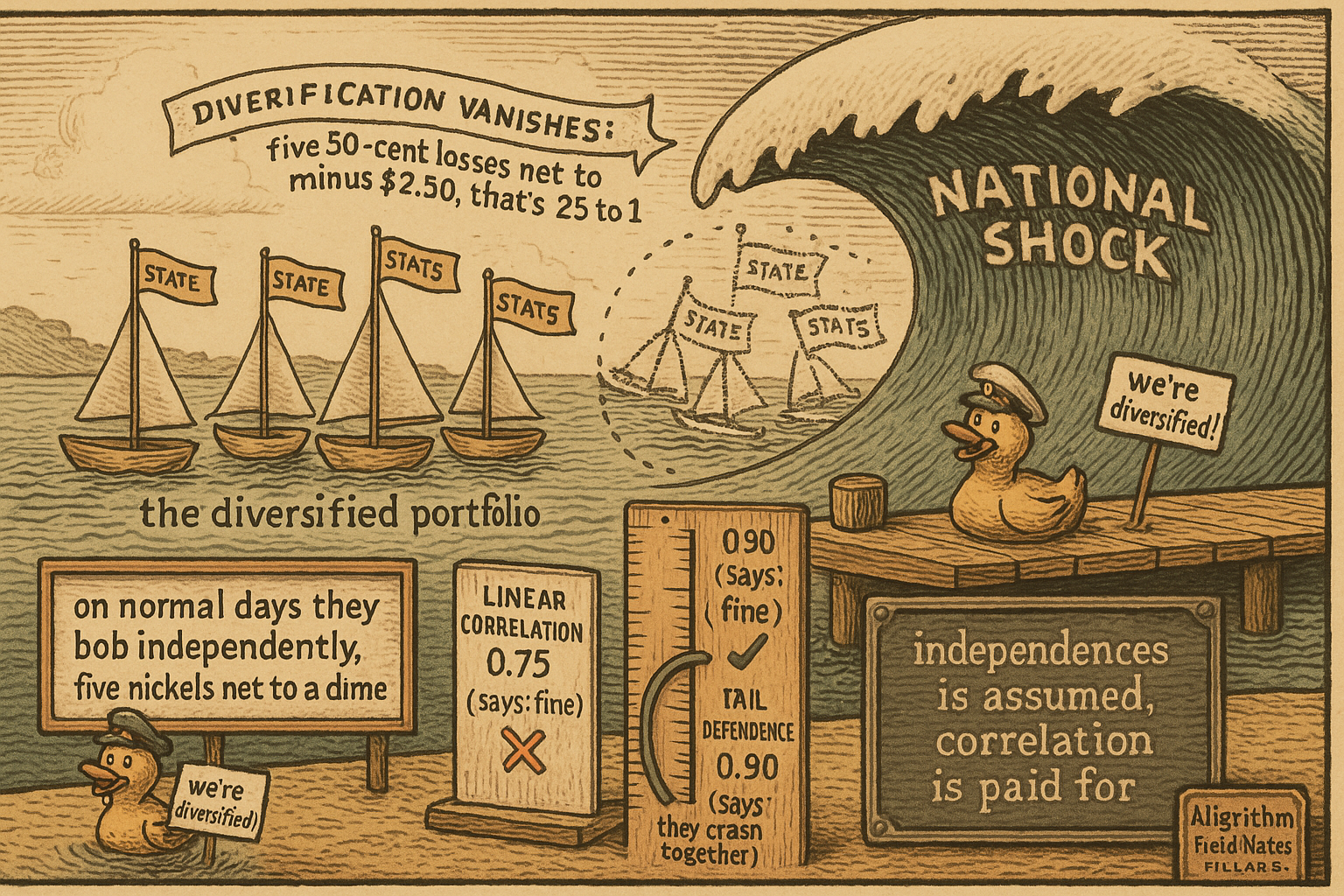
You hold arbitrage positions across five US state-election markets and you feel diversified. Five separate markets, five separate resolutions, the losses should wash out. Then a national-level shock hits, a debate implosion, a scandal, a macro print, and all five markets move the same direction at once. The diversification you counted on evaporates precisely when you needed it, and the portfolio that was supposed to lose a dime loses two and a half dollars. The linear correlation number on your dashboard said 0.75 and looked manageable. It was measuring the wrong thing. Correlation describes how markets move together on an average day. It says almost nothing about how they move together on the worst day, and the worst day is the only one that can end you.
This is anti-pattern number four from "The Six Ways to Lose Money on Polymarket" written out in full. That article named correlation blindness as a way to blow up; this one gives you the math that separates the average-day co-movement you can ignore from the bad-day co-movement that bounds your real downside, and the tool, a copula, that lets you size for the second instead of the first.
Correlation understates the tail
The linear correlation coefficient between two election markets might be 0.75. That describes the ordinary scatter, how the two returns track each other across the full cloud of normal days. What you actually care about is a different quantity, the tail dependence coefficient, which asks a sharper question.
$$ \lambda_{\text{upper}} = \lim_{q \to 1} \Pr\!\bigl(Y > F_Y^{-1}(q) \,\big|\, X > F_X^{-1}(q)\bigr) $$
Read that as: given that market X just had an extreme move, past its q-th percentile with q pushed toward 1, what is the probability that market Y also had an extreme move? That conditional probability, in the limit at the very edge of the distribution, is the tail dependence. Linear correlation averages over the whole distribution and drowns this out. Two markets with correlation 0.75 can carry tail dependence of 0.85 to 0.95, meaning that when one goes to an extreme the other almost always follows. A risk model built on the 0.75 alone underestimates the joint extreme loss by a factor of three to five, which is the exact gap between the loss you budgeted for and the loss that shows up.
The old article "Fat Tails: Why Gaussian Thinking Breaks Trading Systems" makes the univariate version of this mistake: assume a normal distribution and the extremes that actually drive your P&L are dismissed as impossible. Tail dependence is the multivariate cousin. It is not that each market has fat tails, it is that their tails are wired together, and a Gaussian view of the joint distribution treats a synchronized five-market crash as a once-in-the-history-of-the-universe event while the market delivers one every election cycle.
The 25 to 1 blow-up, worked
Put numbers on the five-market portfolio. Under normal conditions each position swings a nickel, and because the day-to-day moves are close to independent you get a genuine diversification benefit, the portfolio swings about a dime, roughly the square-root-of-five shrinkage you would expect. Then the national shock arrives and every position moves adversely at the same time.
| Scenario | Per position | Portfolio | Diversified? |
|---|---|---|---|
| Normal day | plus or minus 5 cents | plus or minus 10 cents | Yes |
| Joint tail (national shock) | minus 50 cents | minus $2.50 | No |
The normal-day row shows real diversification: five independent nickels net to about a dime, not a quarter. The joint-tail row shows it vanishing: five positions each down 50 cents net to $2.50, with no cancellation, because on the bad day they are not five independent bets, they are one bet on the national environment wearing five costumes. The tail-to-normal loss ratio is 25 to 1. An independence assumption would have predicted 5 to 1. The old article "The Death of the Single-System Trader" derives the portfolio-volatility benefit of combining uncorrelated systems, the square-root scaling that makes diversification work, and the lesson here is the sharp edge of that same blade: the benefit is real on normal days and conditional on the correlations staying low, and when a shock drives the correlations to one, the square-root math you were relying on simply does not apply.

A copula separates how each market behaves from how they move together
The fix is to stop modeling the joint distribution as one lump and split it in two. A copula does exactly that: it separates the marginal behavior of each market from the dependence structure that links them.
$$ F(p_1, p_2) = C\bigl(F_1(p_1),\, F_2(p_2)\bigr) $$
Read that as: the joint distribution F of the two prices factors into the individual distributions F-one and F-two, each describing one market on its own, wrapped inside a copula function C that describes only how they move together. You model each market's own behavior however you like, then choose a copula to glue them, and the choice of glue is where the tail dependence lives. This is the same separation the old article "Why Portfolio Construction Is Part of the Signal" argues for at the portfolio layer: the quality of the individual trades and the quality of how you combine them are two different problems, and here the copula is the formal object that carries the combination half.
Gaussian glue hides the crash, Student-t glue shows it
The choice of copula is not cosmetic. Run 10,000 simulated scenarios for the five correlated election markets and count how many produce a joint extreme loss. Under a Gaussian copula you might see about 5 such scenarios. Under a Student-t copula you see 50 or more. Same marginals, same nominal correlation, ten times the joint-tail events, because the Gaussian copula has thin tails and forces extreme co-movement to be rare, while the Student-t copula lets the markets clutch together in the tails the way real correlated markets do under a shock.
For election markets, use a Student-t copula with the degrees-of-freedom parameter around 4 to 6. That setting gives you moderate correlation on normal days and strong co-movement in the tails, which matches how state markets actually behave: loosely linked most of the time, tightly linked when a national event moves everything. The parameter controls how fat the joint tails are. Push it to infinity and you recover the thin-tailed Gaussian copula that just underestimated your risk; drop it to 3 or 4 and you get the heavy, crisis-like dependence seen in stressed financial assets. Around 4 to 6 is the honest middle for election portfolios. This is the modeling engine behind the companion notebook for this pillar, which runs the 10,000-scenario simulation both ways and reproduces the 25-to-1 tail ratio, so you can see the Gaussian model undercount the crashes on your own positions.
Independence is assumed, correlation is paid for
The guideline is one line, and it is the whole chapter: compute portfolio risk with copula-based simulation, not a multivariate-normal assumption, because the chance of simultaneous adverse moves across correlated markets is far higher than a Gaussian model admits. Many individually good trades can combine into a portfolio that dies on a single shock, which means the portfolio-sizing framework from "Kelly Isn't Enough: Drawdown- and CVaR-Constrained Sizing and the Portfolio QP" is incomplete if it feeds on linear correlation. The correlation-risk penalty term in that quadratic program has to be built from the tail-dependence structure, or the optimizer will happily load up five state markets it believes are diversified and hand you the 25-to-1 loss the first time the nation moves as one. Portfolio construction is the seventh source of edge in the hierarchy, a meta-edge that prevents catastrophe rather than generating profit, and the way you earn it is by refusing to assume independence you have not measured, and by pricing the correlation you are actually carrying.
KEY POINTS
- Linear correlation describes average-day co-movement and says almost nothing about the worst day. Two election markets at correlation 0.75 can have tail dependence 0.85 to 0.95, and the worst day is the only one that ends you.
- Tail dependence is the conditional probability that market Y hits an extreme given that market X did, taken at the edge of the distribution. A model using only linear correlation underestimates joint extreme losses by three to five times.
- Worked five-market portfolio: normal days, plus or minus 5 cents per position nets to plus or minus 10 cents (real square-root diversification). National shock, minus 50 cents per position nets to minus $2.50 with no cancellation. The tail-to-normal ratio is 25 to 1, not the 5 to 1 independence predicts.
- A copula separates each market's own behavior (the marginals) from how they move together (the dependence). The choice of copula is where tail dependence lives.
- Gaussian copula versus Student-t on 10,000 scenarios: about 5 joint extreme losses versus 50 or more. The Gaussian has thin tails and forces synchronized crashes to be rare; the Student-t lets markets clutch together in the tails. Use a Student-t with degrees of freedom around 4 to 6 for election portfolios.
- Independence is assumed; correlation is paid for. The portfolio QP must build its correlation penalty from tail dependence, not linear correlation, or it will load up markets it wrongly believes are diversified. This is the portfolio meta-edge: preventing the one-shock blow-up.