9.16 Kelly Isn't Enough: Drawdown- and CVaR-Constrained Sizing and the Portfolio QP

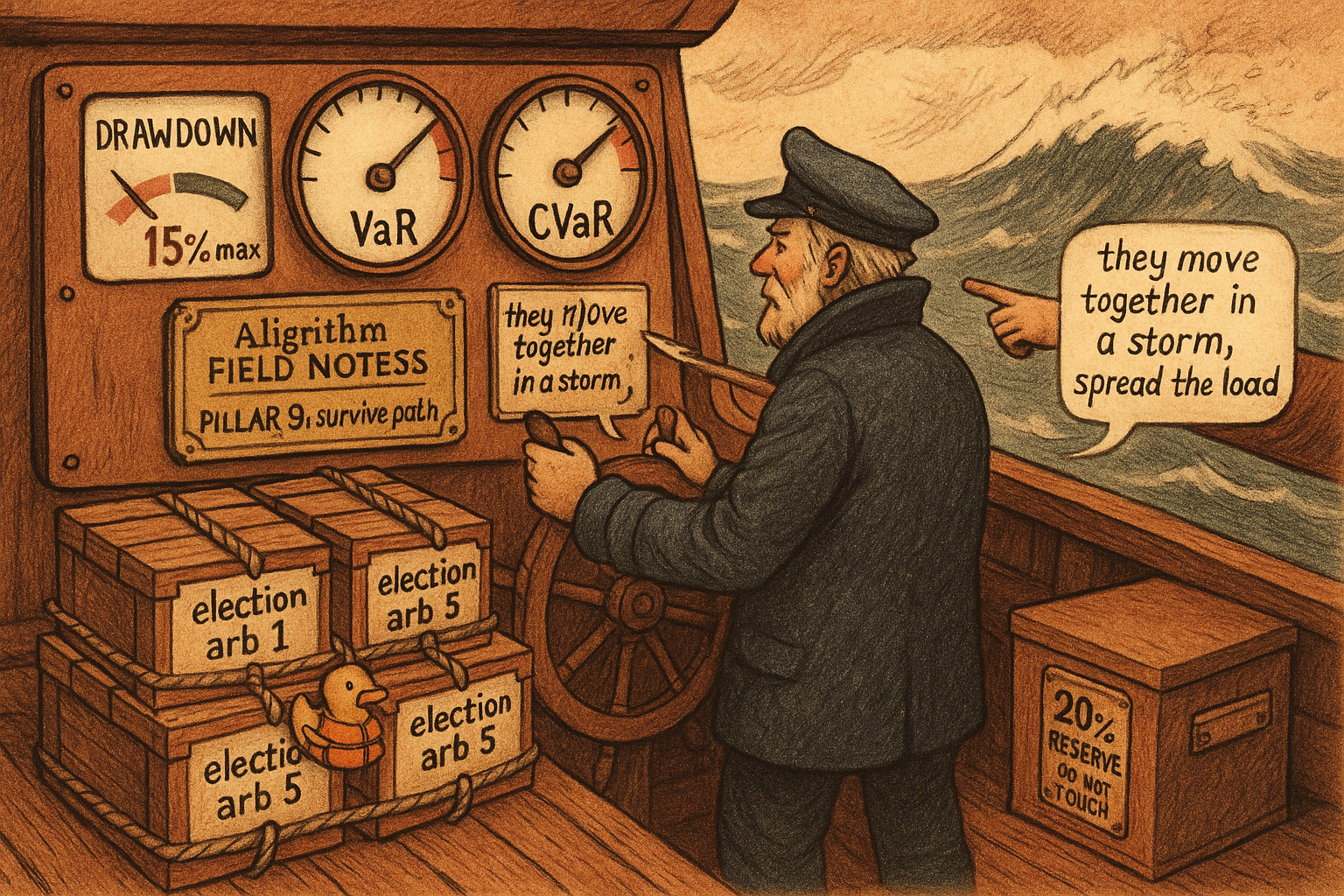
Kelly maximizes growth. It does not promise you survive the path. The article "Kelly Rejects Bad Trades Automatically" ended on the variance buried inside the growth-optimal fraction: a real edge at full Kelly still draws down past 50 percent one time in ten. Growth-optimal and survivable are different objectives, and a trader who optimizes the first without constraining the second gets margin-called out of a winning strategy. This article adds the two constraints that keep you in the game, drawdown and tail risk, and then combines many trades into one allocation that accounts for the way arbitrage positions secretly move together.

Maximum drawdown, and why even optimal strategies bleed

Drawdown is the peak-to-trough drop in your capital, measured as a fraction of the peak.

$$ \mathrm{MDD} = \max_{t_1 < t_2} \frac{W(t_1) - W(t_2)}{W(t_1)} $$

The MDD is the worst such drop over the whole path: take every peak, find the deepest valley that follows it, keep the largest percentage fall. A mathematically optimal strategy still produces ugly ones, because execution fails on some legs, correlated events cluster losses into the same week, and edges decay as competition arrives. None of those show up in the expected growth rate, and all of them show up in the equity curve. The article "Execution Is Part of Expected Value" is where the first cause gets quantified; here the concern is bounding the damage before it happens.

Size to a drawdown budget, by simulation

State the goal as a constraint on Kelly, not a replacement for it. Maximize growth subject to keeping the odds of a drawdown worse than your budget below some tolerance.

$$ \max_f\; G(f) \quad \text{subject to} \quad P(\mathrm{MDD} > D_{\max}) \le \alpha $$

The D-max is the worst drawdown you will accept, say 15 percent. The alpha is how often you will tolerate breaching it. There is no clean formula for the f that satisfies this, so you simulate. Pick a candidate f, generate many wealth paths of realistic length, compute the drawdown of each, and check whether the fraction of paths breaching D-max stays under alpha. Too many breaches, cut f and repeat. Binary-search your way down to the largest f that respects the budget.

The heuristic that falls out of running this against arbitrage-style profit-and-loss profiles is worth carrying.

$$ f_{\text{constrained}} \approx 0.3\text{ to }0.5 \times f^* $$

A 15 percent drawdown budget lands you around a third to a half of full Kelly. Notice this sits right in the fractional-Kelly range from the previous article, reached by a different road. There the argument was estimation error; here it is path survival. Two independent reasons point at the same answer: bet a fraction of Kelly, not the whole thing.

VaR tells you the boundary; CVaR tells you how bad it gets past it

Drawdown constrains the sequence. Tail risk constrains the single catastrophic outcome, and the standard tool most people reach for hides exactly the number that matters.

Value at Risk answers "I will not lose more than this on 95 percent of days." Useful, and dangerous, because it says nothing about the other 5 percent. Conditional Value at Risk answers the question that actually kills you: when you are in that worst 5 percent, how bad is it on average.

$$ \mathrm{CVaR}_\alpha = \mathbb{E}\big[\, \text{Loss} \;\big|\; \text{Loss} > \mathrm{VaR}_\alpha \,\big] $$

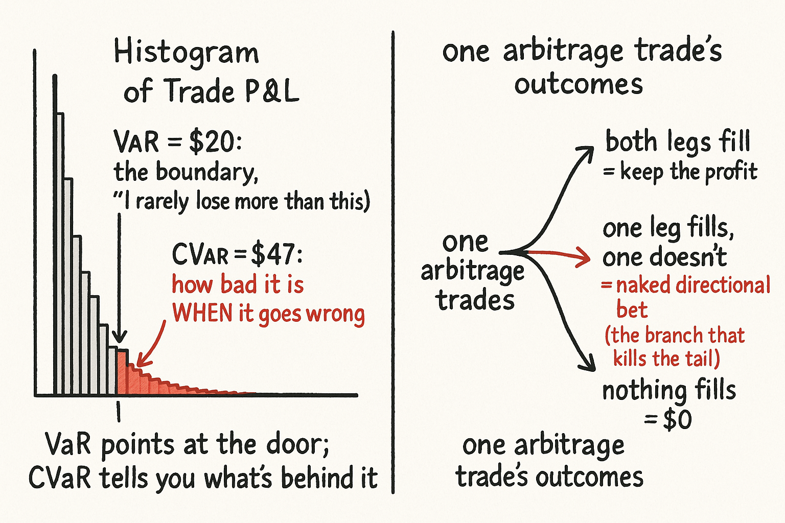
CVaR is the expected loss conditional on being past the VaR boundary. Work the example. Run 100 trades, sort by profit, and the worst five lose 80, 60, 45, 30, and 20 dollars. VaR at 95 percent is 20 dollars, the boundary of the worst five. CVaR at 95 percent is the average of those five, which is 47 dollars.

$$ \mathrm{VaR}_{95\%} = \$20, \qquad \mathrm{CVaR}_{95\%} = \frac{80 + 60 + 45 + 30 + 20}{5} = \$47 $$

VaR reports 20 and calls it a day. CVaR reports 47, more than double, and that is the honest number. The gap is the point: a strategy with a VaR of 20 but a CVaR of 200 has a fat tail that VaR completely conceals, and you find out about it the hard way. Constrain CVaR, not VaR.

For a single arbitrage trade the loss is not a smooth distribution; it has three branches, and the middle one is the dangerous one.

$$ \text{Loss} = \begin{cases} -(\Pi^* - \Delta) & \text{full execution (a small win, or the intended profit)}\\ -(\text{partial cost} - \text{recovery}) & \text{partial execution (the bad branch)}\\ 0 & \text{no execution} \end{cases} $$

Full execution delivers the guaranteed profit. No execution costs nothing but opportunity. Partial execution is where a "risk-free" arb becomes a naked directional position: one leg filled, the other stranded, and you are exposed to the outcome you thought you had hedged. A CVaR constraint exists to stop those partial-execution disasters from dominating your tail, because they are correlated across trades in exactly the moments when everything else is going wrong too.

Many trades, one allocation: the portfolio QP

Sizing trades one at a time misses the thing that blows up arbitrage books: the positions are not independent. Five election arbs that each look clean can all lose together on one national shock. Allocate across all of them at once with a single optimization.

$$ \max_{f_1, \ldots, f_k}\; \sum_i f_i e_i - \tfrac{1}{2}\, \mathbf{f}^\top \Sigma\, \mathbf{f} \quad \text{s.t.} \quad \sum_i f_i \le F_{\max},\;\; 0 \le f_i \le f_i^{\max},\;\; \mathrm{CVaR} \le C_{\max} $$

Read it piece by piece. The first sum is total expected profit, each fraction times its edge. The second term, with the covariance matrix sigma, is a penalty for correlated risk: when two trades tend to lose together, sigma grows and the penalty pushes the allocator to hold less of both, forcing diversification the trader would not do by eye. The constraints cap total deployed capital, cap each individual position, and cap the portfolio's tail loss. This shape is a quadratic program, a squared objective with linear constraints, and standard solvers like CVXPY, Gurobi, or OSQP handle hundreds of trades in milliseconds. The article "Correlation Lies; Tail Dependence Tells the Truth" is where the covariance matrix gets replaced with something that captures joint tails properly, because plain correlation understates exactly the co-movement that matters here.

This is the same QP the production allocator reuses. The article "The Central Allocator and Non-Negotiable Risk Governors" wraps it in a live loop with kill switches; here it is the sizing math underneath.

Priority when capital runs out

Often you cannot fund every good trade. Rank them by profit and confidence per unit of execution risk, and fund from the top.

$$ \text{Priority}_i = \frac{\text{profit}_i \times \text{confidence}_i}{\text{execution\_risk}_i} $$

A high-profit trade with shaky execution ranks below a modest one that fills reliably, which is the correct instinct: guaranteed capture of a smaller edge beats a lottery ticket on a larger one. Allocate down the priority list and keep 20 percent of capital in reserve, because the point of surviving is to have dry powder when the next mispricing appears and the book is not already full.

The through-line across both survival articles is one idea stated twice. Growth-optimal sizing assumes a world with perfect inputs and infinite runway. You have neither. Estimation error argues for a fraction of Kelly, path survival argues for the same fraction, CVaR stops the fat tail you cannot see, and the portfolio QP stops the correlated blowup you did not price. None of it increases your edge. All of it keeps you alive long enough to collect the edge you already have, which the article "Match Your Edge to Your Resources" argues is the whole job once the math is done.

KEY POINTS

• Kelly maximizes growth, not survival. A real edge at full Kelly still draws down past 50 percent one time in ten, so you constrain the path, not just the growth rate.
• Size to a drawdown budget by simulation: pick f, simulate many paths, keep the largest f whose chance of breaching your drawdown limit stays under tolerance. A 15 percent budget lands around 0.3 to 0.5 times Kelly, the same range fractional Kelly reaches from the estimation-error argument.
• VaR reports the boundary of the bad region and hides everything past it. CVaR reports the average loss once you are past it. In the worked example VaR is 20 dollars and CVaR is 47; a VaR of 20 with a CVaR of 200 has a fat tail VaR conceals. Constrain CVaR.
• An arbitrage trade's loss has three branches, and partial execution, one leg filled and the other stranded, turns a risk-free arb into a naked directional bet. CVaR constraints exist to stop that branch from dominating the tail.
• Allocate across all trades at once with the portfolio QP: maximize edge minus a correlated-risk penalty, subject to caps on total capital, per-trade size, and portfolio CVaR. The covariance penalty forces diversification, and QP solvers handle hundreds of trades in milliseconds.
• When capital is scarce, rank trades by profit times confidence over execution risk, fund from the top, and hold 20 percent in reserve. None of this raises your edge; all of it keeps you solvent enough to collect it.

References

• Optimization of Conditional Value-at-Risk - Rockafellar and Uryasev (2000)
• Convex Optimization - Boyd and Vandenberghe (2004)