4. Market Structure Notes June 1, 2026 7 min

4.14 Why Cross-Asset Signals Beat Isolated Chart Reading

One chart is one noisy readout of the macro state. A second market sorts the same days into a better half and a worse half. The lift is small, real, and dies if costs exceed it.

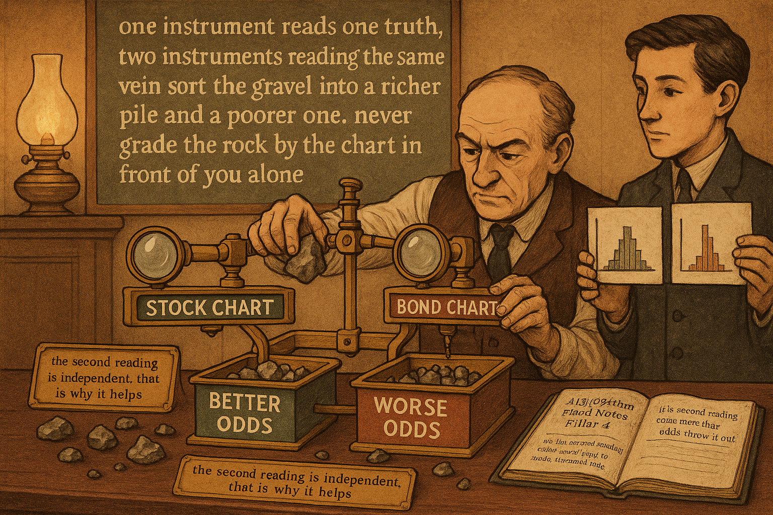
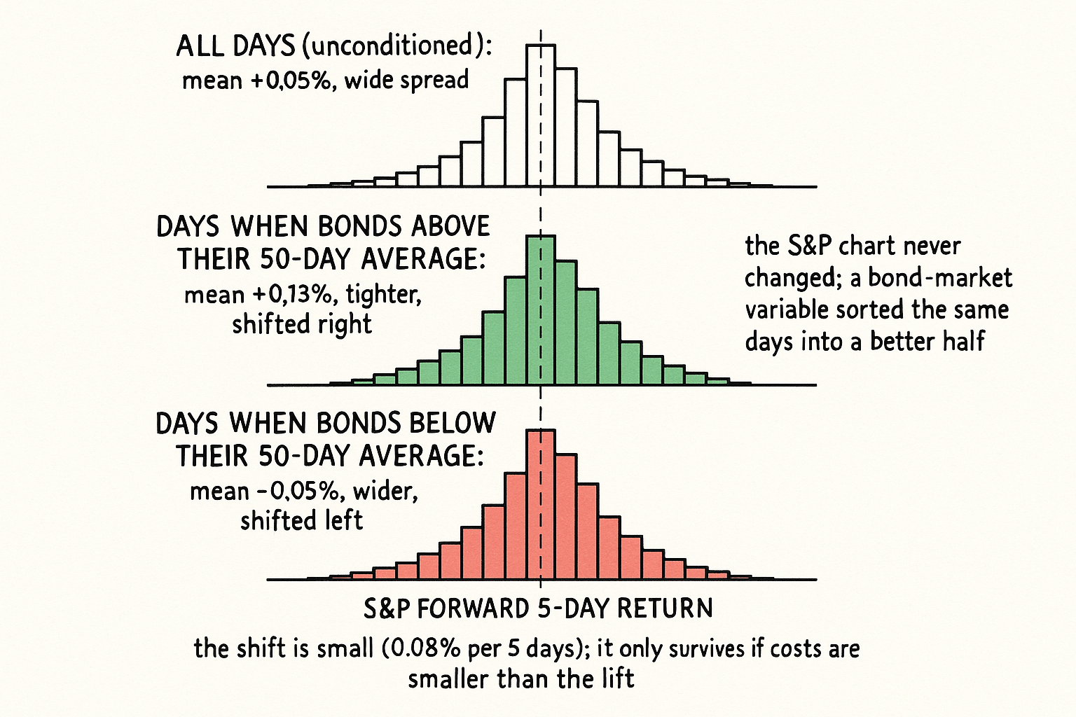
Run a simple experiment on twenty years of S&P 500 daily data. Compute every day's forward five-day return, then split those days into two buckets by a condition that uses no S&P price at all: was the T-bond closing above or below its own 50-day average that day. The full sample might show an average forward return of 0.05% over five days with a standard deviation of 2.0%. Split it, and the "bonds above their average" bucket shows 0.12% with lower dispersion, while the "bonds below" bucket shows 0.00% or slightly negative with higher dispersion. The chart of the S&P never changed. A variable from a different market sorted the same days into a better-expected set and a worse-expected set. That sort is the entire argument for cross-asset signals.

Isolated chart reading uses one information source: the price history of the instrument you trade. Every moving average, breakout level, and oscillator is a transformation of that single series. Cross-asset analysis adds a second, structurally independent source, and the test of whether it helps is mechanical: does conditioning on the external market produce sub-samples with different forward-return distributions than the unconditioned whole. When it does, the external market is carrying tradeable information the chart cannot.

This article makes the case with the distribution-splitting logic, then catalogs when the second source helps and when it is noise dressed as insight. It is the "why" behind the four rule templates from "Intermarket Analysis for System Traders", and it sets up the specific bond-equity filter worked in "Using Bonds to Filter Equity Signals".

The distribution-splitting test

A trading signal is worth something only if it changes the distribution of forward returns relative to the base rate. That standard, borrowed from the way the article "How to Evaluate a Strategy Beyond Net Profit" insisted on looking past a single profit number, is the cleanest way to judge a cross-asset filter.

Start with the unconditioned base rate. For a chosen instrument and horizon, compute the mean, the standard deviation, and the hit rate of forward returns over the whole sample. This is the null: what you get by trading with no filter at all. Then introduce the external condition and recompute the same statistics on each sub-sample.

$$ \text{Lift} = E[r_{t \to t+h} \mid X_t \in \text{state}] - E[r_{t \to t+h}] $$

The lift is the conditional expected forward return given the external market X is in some state, minus the unconditional expected forward return. A positive lift in the "enabled" state and a negative or zero lift in the "disabled" state means the external market is sorting the days into useful buckets. A lift of zero in both states means the external market is decorative, and you have spent degrees of freedom for nothing.

The discipline this enforces: you never accept a cross-asset signal because the story is good. You accept it because the conditional distributions separate, and you reject it when they collapse back onto the base rate. The article "Induction in Trading: Why Past Patterns Are Always Uncertain" applies here in full, because a separation measured on one sample is an estimate, not a guarantee.

Why two sources beat one, structurally

The mathematical reason cross-asset signals can help is that two markets are not perfectly correlated, so the second carries information the first does not contain. If bonds and stocks were correlated 1.0, the bond filter would be a relabeled stock filter and add nothing. They are correlated somewhere around 0.3 to 0.6 over medium horizons, which leaves a large independent component, and that independent component is where the off-chart information lives.

Think of it as two noisy measurements of the same underlying macro state (the level and direction of discount rates, the inflation impulse, the risk appetite of capital). The S&P price is one noisy readout of that state. The bond price is a second noisy readout with different noise. Averaging or cross-conditioning two imperfect readouts of the same latent driver gives a sharper estimate of the driver than either alone, the same logic that makes an ensemble of weak models beat a single one.

The independence is also why the leads exist. Short-rate markets and utility stocks have historically turned ahead of the broad equity market at major inflection points, because they sit closer to the discount-rate driver than equities do. A market closer to the cause moves before a market further down the chain, which is a forward-looking filter rather than a coincident one, and the article "Lead-Lag Relationships in Global Markets" treats measuring that lead as its own problem.

A worked split

Concrete numbers, because the abstract claim does not land otherwise. Suppose 5,000 trading days of S&P forward five-day returns.

Unconditioned: mean 0.05%, standard deviation 2.0%, share of positive days 53%.

Condition on bonds above their 50-day average (roughly 2,800 days): mean 0.13%, standard deviation 1.8%, positive share 57%.

Condition on bonds below their 50-day average (roughly 2,200 days): mean minus 0.05%, standard deviation 2.3%, positive share 48%.

The lift in the "bonds up" state is 0.13% minus 0.05%, equal to 0.08% per five days, with lower dispersion and a higher hit rate. The "bonds down" state has negative lift and higher dispersion. A long-only S&P system that only takes signals while bonds are above their average is trading the better half of the sample and sitting out the worse half. The improvement is not enormous per trade, and that is the honest texture of intermarket edges: small, persistent shifts in a distribution, not a switch between winning and losing.

The annualized arithmetic matters here. An 0.08% improvement per five-day holding period, compounded across the trades you actually take, is the kind of edge that survives only if costs are small relative to it, the constraint the article "Why Transaction Costs Should Be Added Before You Fall in Love" hammered. A cross-asset filter that adds 0.08% and costs 0.10% in extra round-trips is a net loss dressed as an insight.

When the second source is noise

The failure modes, so you do not fool yourself.

The correlation flipped. If your filter was estimated in a regime where stocks and bonds moved together and you trade it in a regime where they move opposite, the lift inverts and the filter actively hurts. The fix is a rolling re-estimate of the correlation sign, and a willingness to disable the filter when the sign is unstable, the slow-drift problem again.

You tested too many external markets. Try thirty candidate markets and you will find one that splits the distribution beautifully on the sample by luck alone. This is the multiple-comparisons trap, and the only honest defense is to fix a small, economically motivated candidate set in advance and count every market you tried, the discipline the article "Optimization Comes After Testing, Not Before" sequenced.

The split is real but tiny relative to costs. A statistically detectable lift that is smaller than your transaction costs is a curiosity, not a strategy. Always net the lift against the extra trading the filter induces before believing it.

Visualizing the split

KEY POINTS

Isolated chart reading uses one information source: the price history of the traded instrument. Every indicator on the chart is a transformation of that single series.
Cross-asset analysis adds a structurally independent second source. The test of whether it helps is mechanical: does conditioning on the external market produce forward-return sub-samples that differ from the unconditioned base rate.
The measure is lift: the conditional expected forward return in a given external state minus the unconditional expected return. Positive lift in the enabled state and zero or negative in the disabled state means the external market sorts days usefully.
Two markets beat one because they are not perfectly correlated (roughly 0.3 to 0.6 over medium horizons), so the second carries a large independent component. Cross-conditioning two noisy readouts of the same macro driver sharpens the estimate.
The independence also produces leads: markets closer to the discount-rate driver (short rates, utilities) turn before equities, giving a forward-looking filter rather than a coincident one.
Worked split: S&P forward five-day return averages 0.05% unconditioned, 0.13% when bonds are above their average, and minus 0.05% when below. The lift is real, small (0.08% per five days), and only survives if costs are smaller.
Failure modes: the correlation sign flips between regimes, you test too many candidate markets and find a fluke, or the split is real but smaller than transaction costs.
The defense: fix a small economically motivated candidate set in advance, re-estimate the correlation sign on a rolling window, count every market tested, and always net the lift against the extra trading the filter induces.