6. Portfolio Construction & System Death July 10, 2026 12 min

6.48 Trend-Following P&L Is a Function of Autocorrelation (Closed Form)

The exact P&L of a European trend-follower is a weighted sum of return autocorrelations plus drift squared. Positive long-horizon autocorrelation pays; the story is optional, the sign is not.

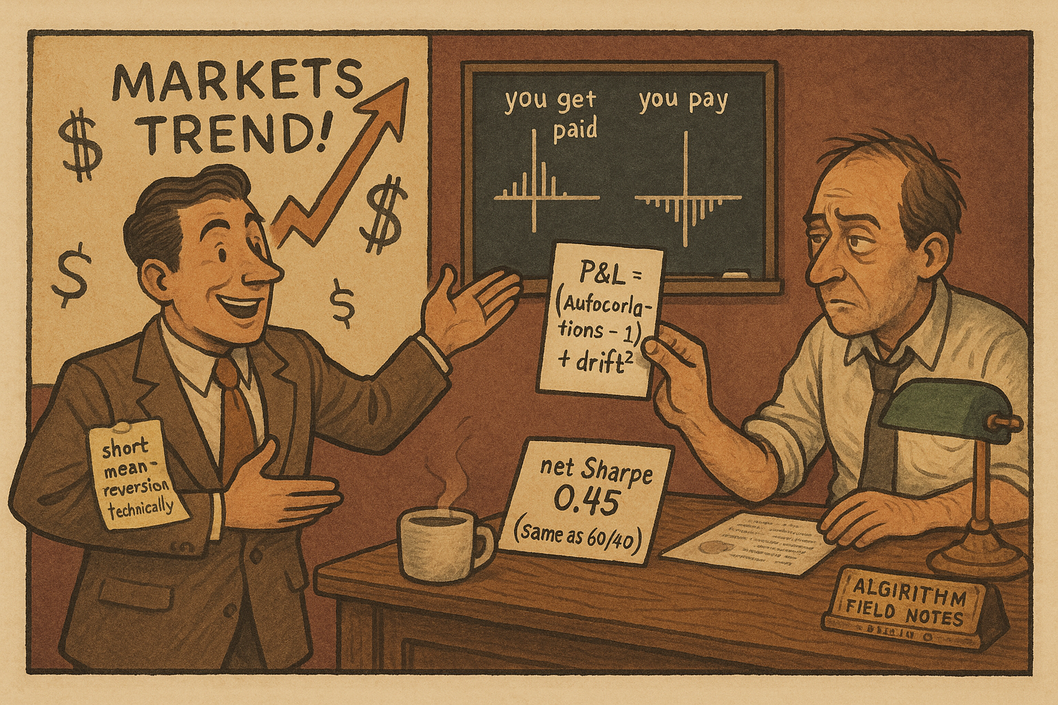
Ask a CTA salesperson why their fund makes money and you get a story: markets trend, we ride the trend, we cut losers and let winners run. That story is untestable. Sepp and Lucic did something the industry rarely does. They wrote down the exact profit-and-loss of a standard European trend-follower and factored it into two things you can measure directly: the autocorrelation of the traded returns and the square of the drift. No story, no hand-waving about market psychology. The whole P&L reduces to one signed number, and if that number is negative the strategy loses no matter how disciplined you are.

The old article "Building a Trend Follower, Component by Component" walked the full construction pipeline: universe selection, a volatility-normalized fast-minus-slow filter, a sigmoid position map, inverse-vol sizing. This piece takes the European branch of that pipeline and asks the harder question. Given the machine is built correctly, what does it actually earn, and on what does that number depend? The answer is a closed form, and it is unforgiving.

The daily return is signal yesterday times return today

Start with what a European trend-follower does on any given day. It holds a position whose size is the smoothed signal times a volatility target, and it earns that position times today's return. Strip the bookkeeping and the daily P&L collapses to a product.

$$ f_t = w_{t-1} r_t = \frac{\sigma_{target}}{\sqrt{a}} \, s_{t-1} \, z_t $$

Read it plainly. The term f-sub-t is the strategy's return today. The s-sub-t-minus-1 is the signal computed through yesterday, an exponentially weighted moving average of past volatility-normalized returns, which you can read as a running estimate of the Sharpe ratio. The z-sub-t is today's return divided by its estimated volatility. Sigma-target over root-a is a constant that just sets the risk level. The strategy return today is yesterday's trend signal multiplied by today's normalized move.

Work a number. Set the annual volatility target to 15%, and the annualization factor a to 260 trading days, so root-a is about 16.1 and the constant is 0.15 divided by 16.1, or 0.0093. Suppose the signal through yesterday sits at 1.5 (a decently strong uptrend on a z-score scale) and today the market delivers a normalized return of 0.8. The day's P&L is 0.0093 times 1.5 times 0.8, which is 0.011, or 1.1%. If today the market instead drops and z-sub-t comes in at minus 0.8, the same positive signal now loses 1.1%. The strategy is betting that a positive signal is followed by a positive return. That bet only pays if returns are positively autocorrelated, and that is exactly what the closed form makes precise.

The whole cumulative return is autocorrelation minus one, plus Sharpe squared

Sum those daily products over a period and the mess of cross terms telescopes into something clean. This is the load-bearing result of the paper, the part the authors flag as new.

$$ \hat{F}_T \propto \hat{\gamma}_T(0)\left(\left[\sum_{m=0}^{\infty} \nu^m \hat{\rho}_T(m) - 1\right] + \frac{\nu}{1-\nu}\frac{(\overline{z}_T)^2}{\hat{\gamma}_T(0)}\right) $$

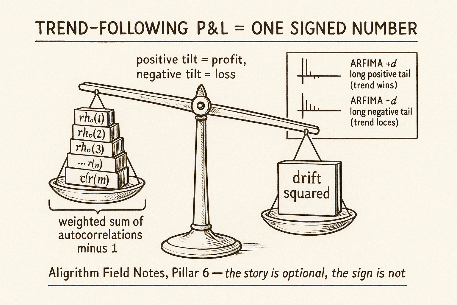
The cumulative return F-hat-sub-T splits into two drivers. The first is a weighted sum of the sample autocorrelations rho-hat at every lag m, with the weight nu-to-the-m shrinking as the lag grows, and then you subtract one. The subtracted one is the lag-zero term, rho(0), which always equals one; it is the price of admission, the cost of trading against your own noise. The second driver is the square of the sample mean of normalized returns over its variance, which is just the squared Sharpe ratio of the underlying.

The subtraction is the whole skeptical point. The weighted autocorrelation sum starts at one because a series is perfectly correlated with itself at lag zero. Subtract that one and you are left with the sum of the genuine forward-looking autocorrelations at lags one, two, three and beyond, discounted by the filter. If those lagged autocorrelations are on balance positive, the bracket is positive and the trend-follower makes money. If they are on balance negative, meaning the market mean-reverts at the horizons your filter cares about, the bracket goes negative and the strategy bleeds. The average autocorrelation must be positive for trend-following to work. Everything else is sizing.

Note what does not appear. The sign of the average return, z-bar, is squared, so a trend-follower is indifferent to whether the drift was up or down. It profits from a strong down-move as readily as a strong up-move, because it can go short. That squared term is why trend-following is a long-volatility, direction-agnostic bet, not a disguised long position.

White noise: no memory, no edge, only drift squared

Feed the formula a process with zero autocorrelation at every nonzero lag, plain white noise with a drift. Every rho(m) for m at least one is zero, so the entire autocorrelation bracket vanishes. Only the drift term survives.

$$ \hat{F}_{1y} = \left(\frac{l\,\sigma_{target}}{\sqrt{a}}\right)\left(\mu^{z}_{an}\right)^{2}, \qquad l = \sqrt{span} $$

The annual return F-hat-1y equals a constant times the square of the annualized drift mu-z-an, which is the Sharpe ratio of the underlying. The loading l for the variance-preserving filter equals the square root of the filter span. Two things fall out. First, without autocorrelation a trend-follower can still make money, but only from drift, and only from its square, so a Sharpe of zero on the underlying gives you nothing. Second, that drift capture scales with the square root of the lookback, so longer filters harvest more of it.

Work it. Take an underlying with an annualized Sharpe of 0.5, so mu-z-an is 0.5 and its square is 0.25. On a one-year span of 250 days, l is root-250, about 15.8, and the annual return is 15.8 times 0.15 divided by 16.1, times 0.25, which is 3.7%. Drop to a one-month span of 21 days and l falls to about 4.6, giving 15.8 becomes 4.6, and the return collapses to roughly 1.1%. Same market, same drift, and the long filter earned more than triple the short one. This is the paper's "drift squared benefits long lookbacks" result stated in dollars: if all you have is a persistent drift and no genuine trending memory, you want a slow system, because a slow system spends more of its time leaning into the drift.

AR(1): the sign of one coefficient decides everything

Now give the process real memory. An AR(1) process has autocorrelation that decays geometrically, rho(m) equals phi-to-the-m, and the infinite weighted sum has a tidy closed form.

$$ \hat{F}_{1y} = c_{1y}\left[\frac{\phi\nu}{1-\phi\nu}\right] + \left(\frac{l\,\sigma_{target}}{\sqrt{a}}\right)\left(\mu^{z}_{an}\right)^{2}, \qquad c_{1y} = l\,\sigma_{target}\sqrt{a}\,\frac{1-\nu}{\nu} $$

The bracket phi-nu over one-minus-phi-nu carries the sign of phi, the autoregressive coefficient. Positive phi means today's return tends to follow yesterday's, a diverging or trending market, and the bracket is positive. Negative phi means returns reverse, a mean-reverting market, and the bracket goes negative. The drift term on the right is unchanged from the white-noise case. The strategy's edge is now literally the sign of a single autocorrelation parameter.

Take a one-month span, 21 days, so nu is 1 minus 2 over 22, about 0.909, and l is root-21, about 4.58. With a modest phi of 0.05 and zero drift, the bracket is 0.05 times 0.909 over one minus that product, which is 0.0455 over 0.9545, about 0.0476. The constant c-1y works out near 1.11, so the annual return is about 5.3%. Flip phi to minus 0.05 and every term keeps its magnitude but the bracket turns negative, so the same system loses about 5% a year on the same volatility. Nothing changed except whether the market trended or reversed at the daily scale.

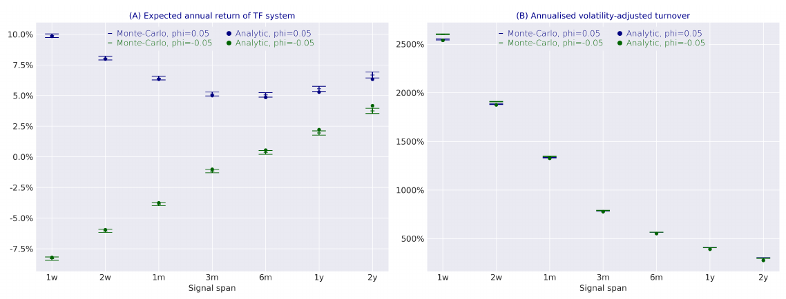
Expected annual trend-following return and turnover as a function of filter span, for a mildly trending AR(1) process (phi = 0.05) and a mildly mean-reverting one (phi = -0.05)

The left panel is the mirror image the theory predicts: the phi equals 0.05 curve sits entirely above zero and its phi equals minus 0.05 twin sits entirely below, roughly symmetric around it. There is also a lesson about span. For a trending market the return is highest at the shortest spans and decays as the filter slows, because a short filter reacts fast enough to ride short-lived momentum. For a mean-reverting market the loss is also deepest at short spans. The takeaway from the old article "Trend and Reversion Are the Same, and OLS Understates Both" lands here with a vengeance: trend and reversion are one process read at two signs of phi, and the same closed form prices both. A trend-follower is a short-mean-reversion position and nothing more.

ARFIMA: trend can win even when the short term reverses

Real markets are not AR(1). They mean-revert over days and trend over months, and a one-parameter model cannot hold both. The paper reaches for the fractionally-integrated ARFIMA process, which carries a long-memory parameter d controlling how slowly the autocorrelation decays, layered on top of a short-term AR(1) term phi. This is where the result earns its keep.

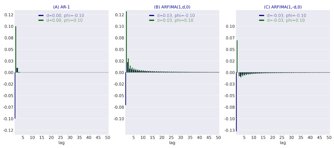
Autocorrelation functions for AR(1) versus long-memory ARFIMA processes: AR(1) dies after a few lags, positive-d ARFIMA keeps a small positive tail out to fifty lags, negative-d ARFIMA keeps a negative tail

Look at the shapes. Panel A, the plain AR(1), spikes at lag one and is dead by lag three; all its memory is short. Panel B, ARFIMA with positive d, has the same short-term spike but then a long, slowly decaying tail of small positive autocorrelations stretching out to fifty lags. Panel C, negative d, keeps a persistent negative tail. Now recall the closed form: the trend-follower sums nu-to-the-m times rho(m) over every lag. Even when the lag-one autocorrelation is negative (short-term reversion, the blue phi equals minus 0.1 line), a long positive tail from a positive d can outweigh it once you use a slow enough filter that reaches those far lags.

That is the paper's most useful and least intuitive claim, and it drops straight out of the arithmetic. A market can reverse day-to-day and still be a profitable trend-following market, provided it trends over the long horizon and you run a slow filter. The weighted sum is what matters, not any single lag. Conversely, with negative d the long tail is negative and even a positive drift only rescues the strategy if the drift is large and the span is long. The formula turns "does trend-following work here" from a vibe into an integral you can evaluate against a process's autocorrelation function.

This is the measurable version of the rhyme from the old article "Why the Market Does Not Repeat, But Still Rhymes." The rhyme a trend-follower harvests is not a chart shape you eyeball; it is the sign of a discounted sum of autocorrelations. If that sum is positive at your horizon, the market rhymes in your favor. If it is negative, no amount of discipline saves you.

Turnover is fixed by the span, not the market

One more result, because it decides whether any of the above survives costs. The expected volatility-adjusted turnover of the European system depends only on the filter span, not on the return process at all.

$$ \mathbb{E}[a\,U_t] = \frac{2a}{\sqrt{\pi}}\,\sigma_{target}\,\sqrt{1-\nu}, \qquad 1-\nu \approx \frac{2}{span} $$

The expected annual turnover is proportional to root of one-minus-nu, which is proportional to one over the square root of the span. Halve nothing about the market; just shorten the filter and turnover, and therefore cost, climbs. For a one-month span, one-minus-nu is about 0.091 and the formula gives roughly 1300% annualized volatility-adjusted turnover. Stretch to a three-month span and it falls to about 780%. The right panel of the AR(1) figure confirms it: turnover decays with span regardless of phi.

Here is the squeeze. Short filters capture short-term trending better (higher gross return when phi is positive) but they trade far more (higher cost). The paper's grid backtest lands on a long span of 250 and a short span of 20 as the practical optimum, where realized costs run about 1.7% a year, in line with a real CTA. Push faster and costs eat the extra gross. That trade-off is not a market opinion; it is baked into these two formulas.

Does the closed form survive real data

A clean formula is worthless if the market's autocorrelation is too small to beat costs, so the honest question is the size of the effect. The paper runs all three systems on a broad liquid-futures universe. Net of transaction costs and a 2-and-20 fee load, the European, American, and TSMOM systems and the SG Trend index all cluster around a Sharpe of 0.45 from 2000 to 2025, the same as a plain 60/40 stock-bond portfolio. On the longer sample back to 1965 the net Sharpe is about 0.63. These are not spectacular numbers. The genuine long-horizon autocorrelation in futures is real but thin, exactly what the discounted-sum formula would tell you to expect from a market that is mostly efficient.

The value shows up somewhere else. All three systems are near-uncorrelated with 60/40 over the full sample but strongly anticorrelated in the worst quarters, so almost all of their Sharpe is earned in the bear regime. Blend 40% into a 60/40 book and the combined Sharpe roughly doubles to about 0.9 while the bear-regime drawdown collapses. Adding portfolio volatility targeting lifts the European system's long-run Sharpe from 0.77 to 1.12, at the cost of some positive skew. The closed form explains why: the payoff is convex and direction-agnostic because the drift enters squared, which is exactly the profile you want as a hedge against a long-only portfolio, not as a standalone alpha engine. Trend-following is a diversifier that happens to be free-standing, priced by the sign of an autocorrelation sum. Read that way, the modest Sharpe is a feature, not a disappointment.

KEY POINTS

A European trend-follower's daily return is yesterday's signal times today's normalized return, so the strategy is a pure bet that positive signals precede positive returns.
The exact cumulative P&L factors into two drivers: a filter-weighted sum of the return autocorrelations minus one, plus the squared Sharpe of the underlying. The subtracted one is the cost of trading your own noise.
Trend-following makes money only when the average autocorrelation at your filter's horizons is positive. The sign of that sum, not any story about trends, decides the outcome.
Drift enters as its square, so the strategy is direction-agnostic and long-volatility; it profits equally from strong up and down moves, and longer lookbacks capture more of the drift.
Under white noise the edge is purely drift-squared and grows with the square root of the span. Under AR(1) the sign of the single coefficient phi flips profit to loss and back.
Under long-memory ARFIMA a market can mean-revert day-to-day and still be a profitable trend market, if it trends over long horizons and you run a slow filter, because the weighted autocorrelation sum can stay positive even when the first lag is negative.
Turnover depends only on the span, scaling with one over the square root of the lookback, which forces the trade-off between capturing fast trends and paying costs. The paper's optimum is a long span near 250, short near 20, at about 1.7% annual cost.
Net of fees the real edge is a Sharpe around 0.45, no better than 60/40 on its own, but its bear-regime, convex, uncorrelated payoff nearly doubles a 60/40 Sharpe when blended. It is a diversifier, not an alpha machine.

References

A note on AI. The ideas, research, analysis, and conclusions in this article are my own. I use AI tools to help with editing and wordsmithing, because English is not my first language, and I am not shy about that. AI-generated ideas and AI-assisted writing are not the same thing: the first is empty slop from a generic prompt, the second is a tool for communicating years of real research more clearly. Judge the work by its substance, not by whether software helped polish the prose.