2.32 The Transfer Function View: Characterizing Any Indicator with the Z-Transform
Write any linear indicator as a transfer function H(z), a ratio of two short polynomials, and its full behavior reads out: gain at every cycle, lag in bars, and the poles that make it ring.
The old article "Why Traders Should Analyze Indicators Mathematically" made the claim that every common indicator is a known signal-processing operation, and the old article "The Frequency Response of Trading Indicators" showed that the magnitude curve tells you which cycles an indicator keeps or kills. Neither showed you the machine that produces that curve. The transfer function is that machine. Write any linear indicator as a transfer function and you can read its entire behavior, the gain at every cycle, the lag at every cycle, and the resonances that make it ring, straight off one compact fraction, before you ever plot a single bar.
The delay operator: one symbol does the bookkeeping
Start with the exponential moving average, because its recursion contains the one moving part you need. Today's EMA is a slice of today's price plus the rest of yesterday's EMA.
$$ y[t] \;=\; \alpha\, x[t] \;+\; (1-\alpha)\, y[t-1], \qquad \alpha = \frac{2}{M+1} $$
The alpha sets how hard the filter leans on the new bar versus its own history, and the length M maps to alpha through the usual relation. Writing "yesterday's value" as y[t-1] over and over gets clumsy once filters reach across several bars, so engineers compress it into one symbol, the delay operator z to the minus one, which means nothing more than shift back one bar.
$$ z^{-1}\, x[t] = x[t-1], \qquad z^{-2}\, x[t] = x[t-2] $$
Multiply a series by z to the minus one and you get its value one bar ago. That is the whole meaning of z at this stage, a relabeling that turns recursions into algebra. The old article "DSP and Digital Filters for Traders: The Primer Nobody Wrote First" introduced this button; here it earns its keep.
Divide output by input and you get the indicator's DNA
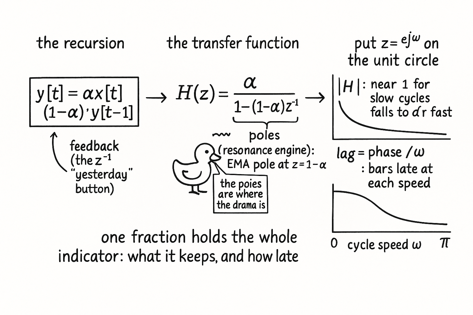
Rewrite the EMA with the delay operator, gather the output terms on one side, and divide output by input. The result is the transfer function, written H of z.
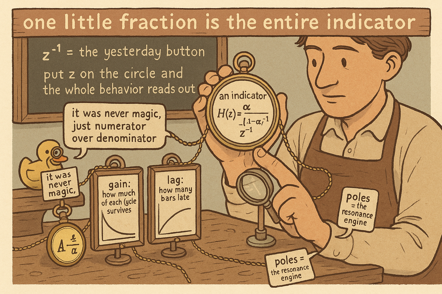
$$ y\,\big(1 - (1-\alpha) z^{-1}\big) = \alpha\, x \qquad\Longrightarrow\qquad H(z) = \frac{y}{x} = \frac{\alpha}{1 - (1-\alpha)\, z^{-1}} $$
That fraction is the complete EMA. The numerator carries the input terms, the denominator carries the feedback terms, and every linear indicator in this pillar reduces to a ratio of two short polynomials in z. The values of z that zero the numerator are the zeros, the cycle speeds the filter kills. The values that zero the denominator are the poles, the feedback resonances that let a recursive filter get a sharp response from almost no storage. The EMA has one pole, sitting at z equal to one minus alpha. A pole near the unit circle makes the filter ring at the matching speed, which you want in a band-pass and nowhere else.
Put z on the unit circle and the frequency response falls out
The transfer function becomes the frequency response the instant you restrict z to the unit circle, setting z equal to e to the j-omega, where omega is the cycle speed in radians per bar. Substitute and split into size and angle.
$$ |H(\omega)| = \frac{\alpha}{\sqrt{1 - 2(1-\alpha)\cos\omega + (1-\alpha)^2}}, \qquad \phi(\omega) = \tan^{-1}\!\frac{-(1-\alpha)\sin\omega}{1 - (1-\alpha)\cos\omega} $$
The magnitude is the gain curve from the old frequency-response article, derived rather than asserted: it sits near 1 for slow cycles where omega is small, and falls toward alpha as omega climbs to pi, the textbook low-pass shape. The phase is the delay each cycle suffers. Turn the phase into the number traders care about, lag in bars, by dividing the phase by the cycle speed.
$$ \text{lag in bars}(\omega) = \frac{\phi(\omega)}{\omega} $$
Now you can answer, for one filter, the two questions that decide whether to use it: how much of each cycle survives, and how many bars late each cycle arrives. Both come from the same fraction, with no backtest and no plotting. That is the payoff of the transfer-function view: the indicator's full character is in H of z, and the unit circle reads it out.
What this buys you, and where it stops
The real leverage shows up when you compose filters. Cascade two filters and you multiply their transfer functions; subtract one output from another, as a moving-average difference does, and you add or subtract the transfer functions. Build a band-pass by placing poles near the cycle you want and zeros at zero and at the Nyquist speed, and the magnitude curve obeys before you write a line of code. Stacking indicators that share a pole-zero layout stacks the same filter, which is the structural reason the redundancy the old frequency-response article warned about exists: confluence between two indicators with the same H of z is one indicator counted twice.
The method has a hard boundary. The transfer function exists only for linear filters, the ones that are a weighted sum of past inputs and past outputs. RSI, stochastics, and anything with a division or a range-normalization are nonlinear, so they have no single H of z, and you can only characterize their linear core before the nonlinear squashing. And a clean transfer function is a description of behavior, not evidence of edge. A filter can pass exactly the band you wanted, with the lag you accepted, and still feed your model a band that carried no predictive value on your instrument. The transfer function tells you what the indicator does. Whether what it does pays is a separate question you answer with data.
KEY POINTS
- The old article "Why Traders Should Analyze Indicators Mathematically" said every indicator is a signal-processing operation; the transfer function is the machine that produces the frequency response the old article "The Frequency Response of Trading Indicators" told you to read.
- The delay operator z to the minus one means shift back one bar. It turns a recursion into algebra so you can manipulate filters as fractions.
- Divide output by input and you get the transfer function H of z, a ratio of two short polynomials. The numerator's roots are zeros (cycles killed); the denominator's roots are poles (feedback resonances). The EMA has one pole at z equal to one minus alpha.
- Restrict z to the unit circle (z equals e to the j-omega) and the magnitude gives the gain at each cycle while the phase gives the delay. Divide phase by cycle speed to read lag directly in bars.
- Composition is algebra: cascade filters by multiplying transfer functions, subtract outputs by subtracting them. Two indicators with the same pole-zero layout are one filter, which is why stacking them is redundancy, not confirmation.
- The method covers linear filters only. RSI and stochastics are nonlinear and have no single H of z. And a clean transfer function describes behavior, never proves edge; whether the passed band pays is an empirical question.
References
- Statistically Sound Indicators for Financial Market Prediction - Timothy Masters (Amazon)
- Cycle Analytics for Traders - John Ehlers (Amazon)
- Introduction to Digital Filters: The Z Transform (Julius O. Smith, Stanford CCRMA)
- The Scientist and Engineer's Guide to Digital Signal Processing: Recursive Filters
- The Ideal Lowpass Filter and Frequency Response (Stanford CCRMA)
- Trend Without Hiccups: A Kalman Filter Approach (transfer-function and lag treatment)