6. Portfolio Construction & System Death June 23, 2026 6 min

6.42 Stable Paretian / Fractal Distributions: Infinite Variance Markets

Mandelbrot's stable Paretian family fits markets better than the Gaussian: fat-tailed, fractal, with infinite variance that breaks volatility sizing, Sharpe, and every variance-based risk number.

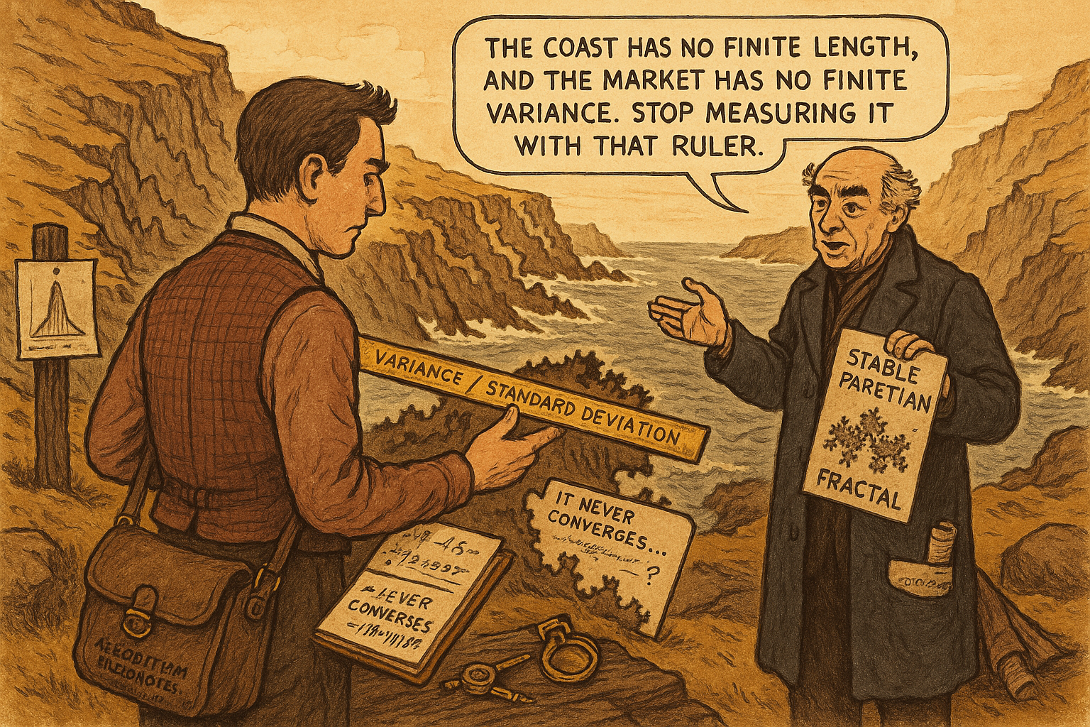
The old article "Lévy Distributions and Market Extremes" introduced the fatter-tailed cousin of the Gaussian and showed where it breaks. Here is the part worth taking seriously, the version Mandelbrot put forward back in the early 1960s when he looked at cotton prices and refused to round the ugly tails off into a bell curve. He proposed that speculative price changes follow a family he called stable Paretian: a sharper peak than the Gaussian, genuine power-law tails, a built-in tendency to trend and to cycle, discontinuous jumps, and one property that quietly demolishes most of the risk math people run. The variance is infinite. Not large. Not hard to estimate. Mathematically undefined. The Lévy stable distribution from the old article is this same family under a different name, and the trading consequence of believing it is that half your toolbox stops being valid.

Mandelbrot's family: peaked center, power-law tails, one knob

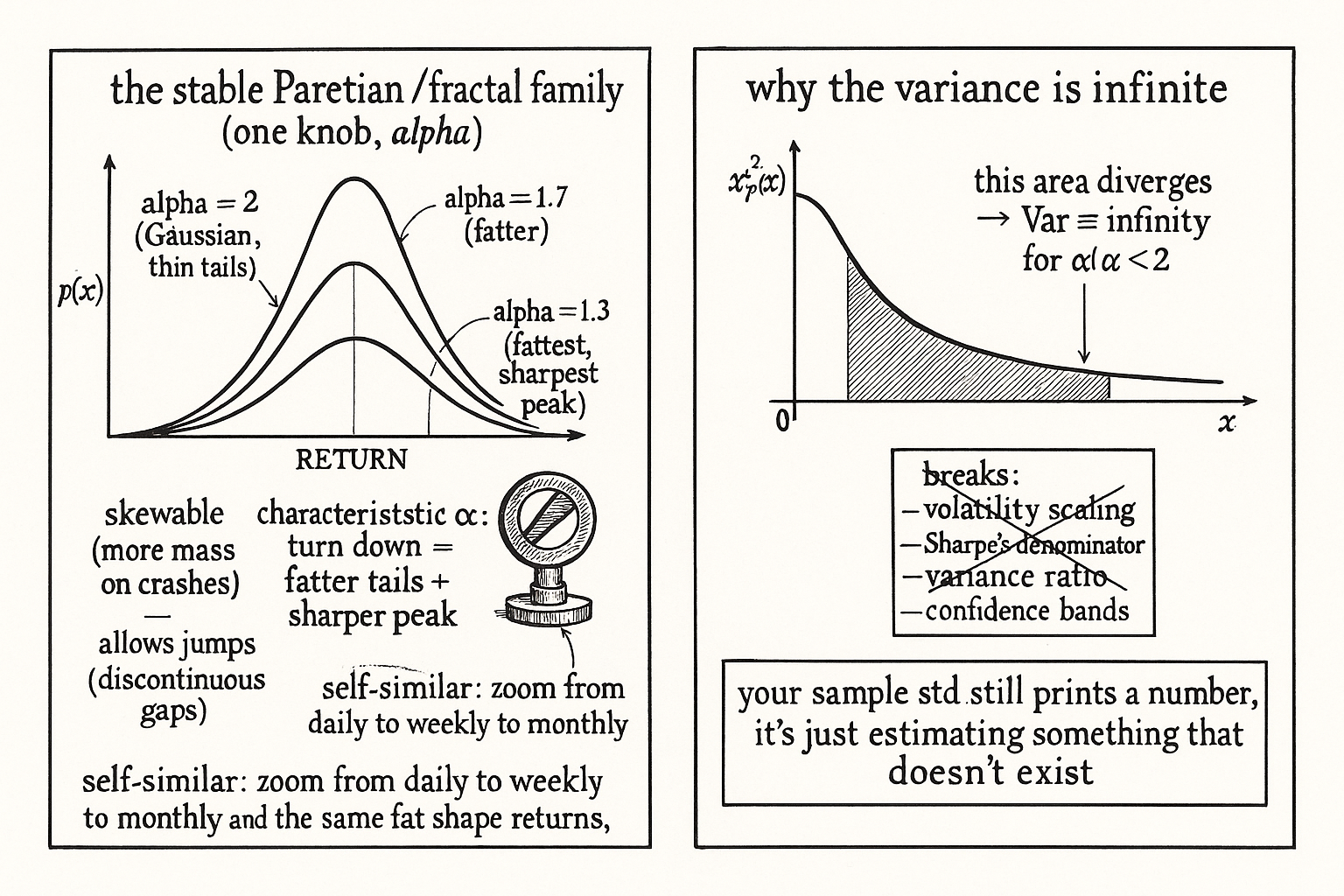
The stable Paretian distributions generalize the Gaussian by adding a single shape parameter, the characteristic exponent, usually written alpha, that controls how fat the tails are. The Gaussian sits at one end of the family with the thinnest possible tails. Turn the knob down and the tails thicken into power laws while the center grows a sharper peak, the leptokurtotic shape real returns show.

$$ P(|r| > x) \sim x^{-\alpha}, \qquad 0 < \alpha \le 2, \qquad \alpha = 2 \Rightarrow \text{Gaussian} $$

The tail probability falls off as the move size raised to a negative power, the slow power-law decay rather than the ferocious exponential decay of the bell curve. A smaller alpha means fatter tails and more frequent extremes. Set alpha to 2 and you recover the normal distribution as the special, thin-tailed corner of the family. So this does not reject the Gaussian; it is a wider net that contains the Gaussian and also contains the peaked, heavy-tailed shapes the market draws.

The family carries two more properties Mandelbrot needed and that matter for trading. It can be skewed, tilted to assign more mass to crashes than to melt-ups or the reverse, which the symmetric Gaussian cannot do. And it allows discontinuous changes, price jumping from one level to another with nothing in between, which is what a gap or an overnight repricing looks like and what no continuous diffusion produces.

Self-similar across scales: why these are called fractal

The reason this family later got the name fractal is that it scales. The shape of the distribution at one timescale looks like the shape at another, up to a stretch factor, instead of smoothing toward a bell curve the way independent Gaussian increments do.

$$ r(\lambda t) \;\overset{d}{=}\; \lambda^{1/\alpha}\, r(t) $$

The return measured over a stretched window of length lambda times t has the same distribution as the original return scaled by lambda raised to one over alpha. The equals sign with the d over it means equal in distribution, the same statistical shape, not the same number. The practical reading: zoom out from daily to weekly to monthly and you do not see the tails politely shrink into normality, you see the same fat-tailed, peaked, jumpy shape rescaled. For the Gaussian, one over alpha is one half, the familiar square-root-of-time scaling. For a fat-tailed alpha below 2, the exponent is larger, so the extremes grow faster than the square root of time as you aggregate. Trends and cycles persist across timescales rather than washing out, which is the same self-similarity the trend-following edge in the old article "Why Fat Tails Are the Reason Trend Following Works" relies on, now stated as a scaling law.

Infinite variance, and what it breaks

The property that earns this distribution its danger label: for any alpha below 2, the variance is infinite.

$$ \text{Var}(r) = \int_{-\infty}^{\infty} x^2\, p(x)\, dx \;=\; \infty \quad \text{for } \alpha < 2 $$

Variance is the integral of the squared deviation weighted by its probability. With power-law tails that decay slowly, the squared term grows faster than the probability shrinks far out in the tail, so the integral does not converge to a finite number. It diverges. This is not a measurement problem you fix with more data. The population quantity does not exist, and the more data you collect the more your sample variance jumps around instead of settling, because the next observation can be large enough to dominate everything before it.

Sit with what that destroys. Any tool that assumes a finite, stable variance is operating on a quantity the distribution refuses to provide. The volatility scaling behind position sizing, the standard deviation in a Sharpe ratio, the variance ratio test from the old article "Variance Ratio Tests for Traders", the confidence bands you draw around an estimate, all of them rest on a second moment that, under a true stable Paretian world, is not there. Your sample standard deviation still computes a number. It estimates something that does not converge, so it understates the risk during calm stretches and lurches when a tail event lands, which is the same instability the old article on fat tails warned makes volatility estimates untrustworthy.

How to use a distribution you cannot trust

You do not adopt the stable Paretian distribution as your working model and start sizing positions off it, for the same reason the old article on Lévy distributions gave: it fits the body and shoulders well and still misses the genuine crashes, and a model with infinite variance is awkward to plug into any sizing formula. Its value is diagnostic, not predictive. It tells you that the trending-and-cyclical, jumpy, scale-invariant character of markets is the baseline, not an anomaly, so you should expect persistence across timescales and stop being surprised by gaps. And it tells you, hard, to distrust every statistic that assumes a finite variance without admitting it. When your risk number is a multiple of a standard deviation, you are leaning on a quantity that may not exist, so treat it as a floor on risk rather than a measure of it, and stress-test against moves larger than any variance-based bound would suggest. The honest takeaway from Mandelbrot's family is not a better curve to fit. It is a warning that the second moment, the thing half of quantitative finance is built on, may be a fiction in the markets you actually trade.

Visualizing infinite variance

KEY POINTS

Mandelbrot proposed in the early 1960s that speculative prices follow a stable Paretian family: a sharper peak than the Gaussian, genuine power-law tails, skewness, and discontinuous jumps. It is the same family as the Lévy stable distribution from the old article "Lévy Distributions and Market Extremes."
One shape parameter, the characteristic exponent alpha, controls tail fatness. At alpha equal to 2 you recover the Gaussian as the thin-tailed corner; turn it down and the tails fatten into slow power laws while the center peaks.
The family is self-similar across timescales, which is why it is called fractal: aggregate from daily to weekly to monthly and the fat, peaked, jumpy shape rescales instead of smoothing into a bell curve, so trends and cycles persist across scales.
For any alpha below 2 the variance is infinite, not large but mathematically undefined, because the slow power-law tail makes the integral of squared deviations diverge. More data makes the sample variance jump around, not settle.
Infinite variance breaks every tool that assumes a finite second moment: volatility-based position sizing, the Sharpe denominator, the variance ratio test, and any confidence band. The sample standard deviation still prints a number, but it estimates a quantity that does not converge.
The distribution is diagnostic, not a working model. It fits the body and misses the crashes like the old article on Lévy showed, so use it to expect persistence and jumps, distrust variance-based risk numbers, and stress-test beyond any bound built on a standard deviation.