10.22 Ranking Beats Forecasting — But Ranking What?

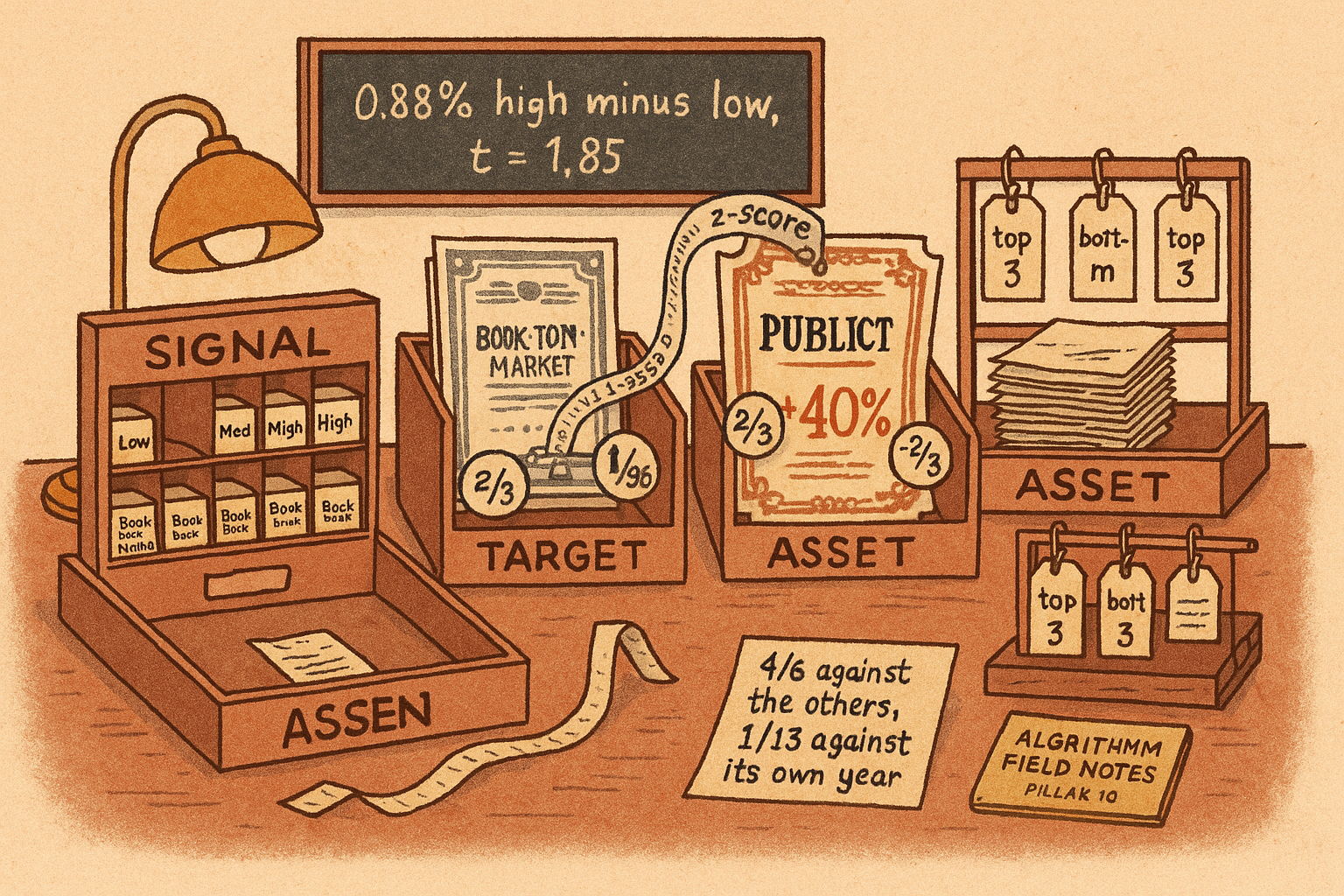
You sort every name in a cross-section and hold the extremes. Chuan Shi's portfolio-sort lecture, Nusret Cakici and Adam Zaremba's target transforms, and Tom Burdorf's LambdaMART portfolios apply that cut to three different objects: the characteristic, the next return, and the asset. Shi ranks book-to-market and cuts ten groups. Cakici and Zaremba replace next month's excess return with its cross-sectional rank, mapped from -1 to +1, and only then fit a model. Burdorf trains on the order of names and keeps the top three and the bottom three. Put one asset's own history into the same percentile formula and the short leg has nobody left to short.

A decile sort ranks the characteristic

The old article "Portfolio Sorts From Scratch: Deciles, Monotonicity, and the Long-Short Spread" builds the sort engine. The object inside the rank is the characteristic. The return is what you measure after the cut. At each month you order the names by a sorting variable x. In Shi's example x is book-to-market. You cut the order into L groups. The convention is L = 10. The factor return λ_t is the high group's return minus the low group's return that month. The two legs are dollar neutral. You value-weight or equal-weight inside the leg, then you rebalance when the characteristic moves. Academic sorts usually rebalance monthly. A live portfolio often rebalances daily.

$$ \begin{aligned} \hat{\lambda} &= \frac{1}{T}\sum_{t=1}^{T}\lambda_t, \\ \mathrm{s.e.}(\hat{\lambda}) &= \frac{\mathrm{std}(\lambda_t)}{\sqrt{T}}, \\ t &= \frac{\hat{\lambda}}{\mathrm{s.e.}(\hat{\lambda})} \end{aligned} $$

λ-hat is the average high-minus-low return over T months. The standard error divides the sample standard deviation of that series by the square root of T. The t-statistic is the average divided by that standard error, and Shi refers it to a t distribution with T - 1 degrees of freedom because the sample standard deviation already spent one. His Chinese book-to-market sort is value-weighted and monthly. He prints a high-minus-low average of 0.88%, a standard error of 0.47%, a t-statistic of 1.85, and a p-value of 0.07. Divide the printed average by the printed standard error and you get 0.88 / 0.47 = 1.87, not 1.85. The printed high leg is 1.44% and the printed low leg is 0.57%, and 1.44 - 0.57 = 0.87, not the printed spread of 0.88. Keep his 0.88, 0.47, and 1.85. The gap is the size of rounding the monthly series before you divide, or the table is slightly inconsistent. A p-value of 0.07 is a weak argument for a live book. The ladder of the ten bins is a separate question, and it is the one the sort is for.

$$ \rho_s = \frac{\operatorname{cov}(X_r, X_g)}{\sigma_{X_r}\,\sigma_{X_g}} $$

X_g is the group index, 1 through 10, from the low bin to the high bin. X_r is the rank of the ten portfolio average returns. ρ_s is their correlation. It equals 1 when the means rise in lockstep with the sort, and it falls when a bin breaks the ladder. His printed means, in percent, are 0.57, 0.53, 0.57, 0.72, 0.94, 0.90, 1.08, 1.32, 1.21, 1.44. The second bin, 0.53, sits below the low bin. The low bin and the third bin both print 0.57, so they share the average rank 2.5. With that tie rule, ρ_s = 0.954. The sort is almost monotone. The premium is noisy. You can have a clean ladder and still fail a funding hurdle.

One characteristic rarely arrives alone. If every high book-to-market name is also a large cap, the high-minus-low book is long size at the same time. The fix is a second rank. An independent double sort cuts each variable into its own groups, usually quintiles, so L_1 = L_2 = 5 and you have 25 portfolios. The factor for the first variable averages the high row and subtracts the average of the low row. The columns are the second variable, which you are holding roughly fixed.

$$ \lambda_{X_1,t} = \frac{1}{L_2}\sum_{i=1}^{L_2} R_{L_1,i,t} - \frac{1}{L_2}\sum_{i=1}^{L_2} R_{1,i,t} $$

R_{L_1, i, t} is the return of the high-X_1 portfolio in column i. R_{1, i, t} is the low-X_1 portfolio in that same column. Shi also prints the average of the five within-column spreads, and the two expressions are the same algebra. Look at the bottom row and the top row of the grid. The bottom row is the high rank of X_1. The top row is the low rank. The factor is the average of the bottom minus the average of the top.

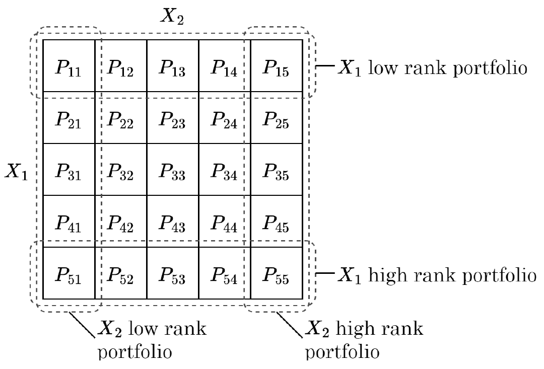
A desk example, not his table. Suppose the five high-row returns are 1.20, 1.10, 0.90, 1.40, and 1.00, and the five low-row returns are 0.40, 0.50, 0.30, 0.60, and 0.20. The high row averages 1.12. The low row averages 0.40. The spread is 0.72 percentage points. The five within-column gaps, 0.80, 0.60, 0.60, 0.80, and 0.80, average to the same 0.72. When the two characteristics move together, the off-diagonal cells (high X_1 and low X_2, or the reverse) hold few names, and one outlier owns that cell. A dependent sort avoids the empty corner: you cut on the control first, then you cut the variable you care about inside each bucket. Only the second variable becomes a factor. The first variable is a control, and you do not average it into its own long-short.

The label is a rank, and the +40 percent month shrinks

The old article "Getting the Target Right: The Transform That Beats 147 Features" runs this horse race on 147 characteristics. The object you recompute here is the label, on one month, before any model is fit. Cakici and Zaremba build every transform inside the month, across the names alive that month.

Five names, excess returns of -8, -1, 0, +2, and +40 percent. The cross-sectional mean is 6.6. They write the cross-sectional standard deviation as σ_t(r) and do not print the divisor. These five names are the whole cross-section, so the divisor is 5, not 4. The deviations from 6.6 are -14.6, -7.6, -6.6, -4.6, and 33.4. The sum of squares is 1,451.2. Divide by 5 and the square root is 17.04 percentage points.

$$ \begin{aligned} r^{DM}_{i,t} &= r_{i,t} - \bar{r}_t, \\ r^{Z}_{i,t} &= \frac{r_{i,t} - \bar{r}_t}{\sigma_t}, \\ r^{Pct}_{i,t} &= \frac{\mathrm{rank}(r_{i,t})}{N_t + 1}, \\ r^{Rank}_{i,t} &= 2\, r^{Pct}_{i,t} - 1, \\ r^{Norm}_{i,t} &= \Phi^{-1}\!\left(r^{Pct}_{i,t}\right) \end{aligned} $$

The demeaned return subtracts the month's cross-sectional mean, so a model cannot fit "this was a bull month" and call it a stock pick. The z-score divides that deviation by σ_t, so a wild month does not dominate the squared error through its scale alone. The percentile divides an ascending rank by N_t + 1. Rank 1 is the worst return in the month, rank N_t is the best, and the best name lands at N_t / (N_t + 1), short of 1. They do not print the tie rule; with no ties the rank is 1, 2, 3, 4, 5 and the denominator is 6. The centered rank stretches that percentile onto [-1, 1]. The Gaussianized rank pushes the percentile through the inverse of the standard normal, which keeps the order and throws away the gaps. Ascending rank is the direction that makes a high return a high label. A descending rank would train the model to buy the losers, and their later decile sort buys the highest forecast.

Walk the +2 percent name through the card. Its demeaned return is 2 - 6.6 = -4.6. Its z-score is -4.6 / 17.04 = -0.27. Its ascending rank is 4, so the percentile is 4/6 and the centered rank is 2 × (4/6) - 1 = 1/3. The inverse normal of 4/6 is 0.43. The same name is a negative z-score and a positive rank label, because the +40 percent name pulled the mean up through +2. A model trained on ranks is told this name beat the cross-section. A model trained on standardized returns is told it finished below the cross-sectional mean.

Walk the +40 percent name. Its z-score is 33.4 / 17.04 = 1.96. Its centered rank is 2 × (5/6) - 1 = 2/3. Its Gaussianized rank is the inverse normal of 5/6, which is 0.97. A name that returned +3 percent and took the same last place would wear the same 2/3 badge. The rank keeps the order and deletes the distance. Gaussianizing the percentile compresses 1.96 down to 0.97. Standardization keeps the distance and lets one name move the mean, which is why the +2 percent name changed sign.

Look at the +2 percent group in the right panel. The z-score bar is below zero. The rank-label bar is above zero. That sign flip is the choice you are making when you pick a target. The left panel is why the z-score looks like that: one +40 percent name owns the scale.

The asset rank keeps three names on each side

The old article "Momentum Is a Ranking Problem: Learning-to-Rank vs Regress-then-Rank" is the squared-error version of this book: fit a return, then sort the fits. Burdorf's LambdaMART step deletes the return from the loss. The score exists so you can order the names. You then keep the extremes and drop the middle.

$$ \begin{aligned} Y^{(i)}_t &= f(\mathbf{u}^{(i)}_t), \\ Z^{(i)}_t &= R(Y^{(i)}_t), \\ S^{(i)}_t &= \begin{cases} -1 & \text{if } Z^{(i)}_t \le 3, \\ +1 & \text{if } Z^{(i)}_t > N_t - 3, \\ 0 & \text{otherwise.} \end{cases} \end{aligned} $$

f reads the feature vector of name i and emits a score Y. The operator R sorts those scores into ascending positions Z, from 1 to N_t. The lowest three scores are shorts. The highest three are longs. Everyone else is flat. On his 16 commodity futures, N_t - 3 = 13, so the longs are positions 14, 15, and 16, and the shorts are positions 1, 2, and 3. On the 29 currency pairs the longs are positions 27, 28, and 29. The holdings ignore whether the top score beat the fourth name by a little or by a factor of ten. That is what ranking the asset does: the magnitude never enters the position.

The holdings then get a volatility weight. He prints the cross-sectional momentum return as an average over the universe, with a target volatility in the numerator.

$$ r^{CSM}_{t,t+1} = \frac{1}{n}\sum_{i=1}^{n} S^{(i)}_t \,\frac{\sigma^{tgt}}{\sigma^{(i)}_t}\, r^{(i)}_{t,t+1} $$

n counts every name in the universe. Names with S = 0 stay in the sum and add nothing, so dividing by the six open positions would overstate the weight. σ^tgt is an annualized target of 15%. σ_t is an ex-ante daily volatility from a 63-day exponentially weighted standard deviation. The fraction does not cancel: an annual number sits on top of a daily number. Take one long commodity with daily volatility 1.2% and a next-day return of +0.8%, inside a 16-name universe. The printed ratio is 0.15 / 0.012 = 12.5, and the name's contribution is (1/16) × 12.5 × 0.008 = 0.625% in a single day. A same-unit daily target is 0.15 / √252 = 0.00945, the ratio falls to 0.79, and the same name contributes about 3.9 basis points. The printed ratio is √252, about 15.87, times a same-unit vol target. He then scales the finished book a second time, so the published series sit near 15% annual volatility. Keep his formula. The ratio sets relative leverage across names. The second scale sets the book's volatility. The 0.625% is an intermediate weight. The reported P&L is the series after the second scale. Treat the unit mix as a possible source error, or as a relative weight that only makes sense before the second scale.

The neural-net benchmark, the regress-then-rank book, trains on the size of the move. He does print that loss.

$$ L(\theta) = \frac{1}{M}\sum_{\Omega}\left(Y^{(i)}_t - \frac{r^{(i)}_{t,t+1}}{\sigma^{(i)}_t}\right)^2 $$

M is the number of name-day pairs in the training window. The target inside the square is next period's return divided by that day's volatility estimate, so the net is fitting a vol-scaled return. Suppose the net emits 0.40, the name returns 1.0%, and daily volatility is 1.2%. The target is 0.01 / 0.012 = 0.833. The squared error on that pair is (0.40 - 0.833)^2 = 0.187, and that pair contributes 0.187 / M to the loss. The net is charged for missing the size. A rank loss is charged for putting this name on the wrong side of another name. Those are different trades. On the +40 percent month from the previous section, squared error charges the z-score of 1.96, and the rank charges the label 2/3.

He writes the learning-to-rank objective as a sum of some loss ℓ on a ground-truth rank y and the model's score, over rebalance dates and names. He does not print ℓ. He says LambdaMART specifies the gradients, which he calls lambdas, directly from a listwise metric, instead of deriving them from a written loss. The lambda expression is not in the paper. The metric he does compute is an average of two normalized discounted cumulative gain scores at three names. Normalized discounted cumulative gain pays more for getting the top of a list right. He scores the top three, scores the bottom three after reversing the true labels, and averages them.

$$ \mathrm{NDCG}_{agg} = \frac{\mathrm{NDCG}^{top}_{3} + \mathrm{NDCG}^{bottom}_{3}}{2} $$

The gain inside that metric is 2 raised to the relevance, minus 1. He does not print the position discount. The usual discount, which his paper does not write down, divides that gain by log base 2 of (position + 1).

$$ \mathrm{DCG}@3 = \sum_{i=1}^{3} \frac{2^{rel_i} - 1}{\log_2(i+1)} $$

A three-name desk calculation, using that usual discount. You ranked relevances 2, 0, 1. The ideal order is 2, 1, 0. Gains are 2^rel - 1, so the ranked list has gains 3, 0, 1 and the ideal list has gains 3, 1, 0. The discounts are log2(2) = 1, log2(3) = 1.585, and log2(4) = 2. Discounted cumulative gain is 3/1 + 0/1.585 + 1/2 = 3.50. The ideal is 3/1 + 1/1.585 + 0/2 = 3.631. The ratio is 3.50 / 3.631 = 0.964. If the bottom three, after the label reversal, score 0.50, the aggregate he prints is (0.964 + 0.50) / 2 = 0.732. Relevance itself cannot go past 31 in the XGBoost build he uses. The gain at relevance 31 is 2^31 - 1 = 2,147,483,647, the top of a signed 32-bit integer, and relevance 32 overflows it. His universes fit under that cap: 16 commodity futures, 18 bond indices, 29 currencies after he drops the Turkish lira, 26 equity indices. A few thousand stocks do not. For that universe you rank the label and then cut deciles. You do not feed a raw rank into a gain of 2 to the relevance.

A percentile down one path has no short leg

The old article "Cross-Sectional Percentile Rank Within a Universe" is the version of this formula whose denominator is a set of names. The old article "Ranking Beats Forecasting for Many Trading Problems" is the claim that this cross-sectional order is the trade. Both formulas below are the same rank. The set inside the rank is the whole difference.

$$ \begin{aligned} p^{CS}_{i,t} &= \frac{\mathrm{rank}_{j \in \mathcal{U}_t}(x_{i,t})}{N_t + 1}, \\ p^{TS}_{i,t} &= \frac{\mathrm{rank}_{\tau \in \{t-L+1,\ldots,t\}}(x_{i,\tau})}{L + 1} \end{aligned} $$

x is the signal you would have sorted on. In a momentum book it is a past return. The cross-sectional percentile ranks that signal against the other names alive at t. N_t is how many names are in the universe. The time-series percentile ranks the same print against the name's own last L observations. L is the lookback, in months here. A momentum sign goes long when the percentile is above one half and short when it is below. A mean-reversion book flips the sign. Either way, the two percentiles can sit on opposite sides of one half, and then the two books take opposite sides.

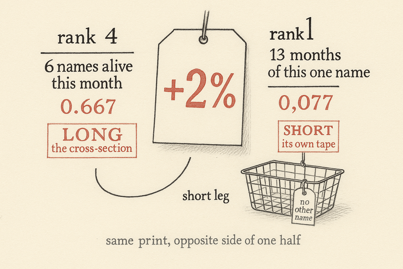
Use the +2 percent name again, and let x be last month's return. Inside the five-name cross-section its ascending rank is 4, so p^CS = 4/6 = 0.667. Above one half: the cross-sectional momentum book is long. Now give that name its own last 12 months, ending at +2: 8, 9, 10, 7, 6, 11, 12, 5, 9, 8, 7, 2. The +2 is the minimum. Its ascending rank is 1, and p^TS = 1/13 = 0.077. Below one half: the time-series book is short. Same print. The denominator changed from 6 names to 13 months. λ_t needs a high group and a low group. This construction has one series, so you are left with the percentile and a sign on that series, sized like any other time-series momentum position.

The label moves the alpha, and the Sharpe barely follows

Look at the percentile bar on the left. That is what happens when you rank the target. The right panel is what happens when you rank the feature instead, and the lift is smaller. Both panels are the averages in Cakici and Zaremba's Figure 1, redrawn from a zero axis. The left bars are average monthly CAPM alphas of a value-weighted high-minus-low decile, in percent, across their feature transforms. CAPM is the capital asset pricing model: the alpha is the intercept after you regress the long-short on the market. The right bars are the same alpha averaged across target transforms, one bar per feature transform.

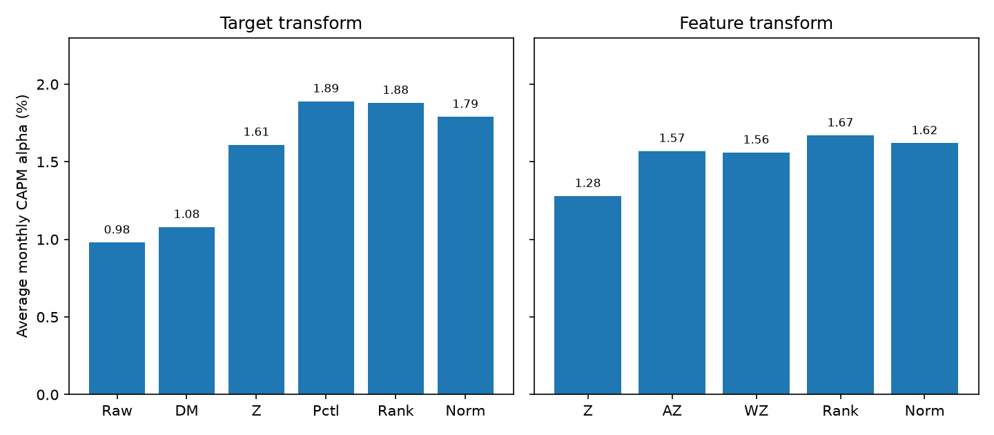
Percentile targets produce a 1.89 monthly CAPM alpha. A raw target produces 0.98. Ranking the feature moves the average alpha from 1.28 on a standardized characteristic to 1.67 on a ranked one. Hold the 1.89 next to the rest of the grid. The percentile column's mean return is 1.61%, and the CAPM alpha on that column is 1.89, so the intercept sits above the average return. Monthly volatility of the long-short averages 3.64% on raw targets and 5.15% on percentile targets. Annualized Sharpe averages 0.89 on raw targets and 1.09 on percentile targets. Check that Sharpe against the column averages: 1.61 × 12, divided by 5.15 × √12, equals 1.08, next to the printed 1.09. The ratio of the averaged inputs is a different operation from the average of the row Sharpes, and here the two land next to each other. The label almost doubled the alpha and added about two tenths to the Sharpe, because monthly volatility rose with it. Equal-weighted books and micro-caps flip the ranking: standardized and demeaned targets earn about 3.15% to 3.16% a month against about 2.57% for rank targets, micro-cap standardized targets earn 3.23% against about 2.99% for ranks, and emerging markets prefer the z-score target at 1.70% against 1.55% to 1.56% for ranks. Developed markets prefer the rank, at 2.11% to 2.15%. Gradient boosting is where the label dominates the model. It rises from roughly 0.2% a month on a raw target to nearly 1.8% once the target is ranked. A forest on raw returns sits near zero, and the ranked target takes it to about 1.4% to 1.5%. Sample frame, gross of costs: 35 markets, 147 characteristics, an eight-model equal-weight ensemble, value-weighted deciles, January 1994 to December 2024, with the test window starting in January 2003.

Burdorf is a different experiment, on a small universe, and the asset-rank result depends on the asset class. Weekly rebalancing, still scaled to about 15% annual volatility, 2000 to 2023, gross: equity LambdaMART Sharpe 0.54, against a neural net at 0.64. Bonds go the other way. The plain 252-day return sort has Sharpe 0.80 and LambdaMART has -0.27. Currencies go further: a random book has Sharpe 0.34 and LambdaMART has 0.20. On the daily grid LambdaMART leads currencies at Sharpe 0.47 and commodities at 0.44, and it trails the neural net in bonds, 1.12 against 1.98. The daily equity Sharpe he prints is 3.40. Divide the printed equity mean of 0.53 by the printed volatility of 0.16 and you get 3.31, not 3.40. Keep 3.40 as his reported Sharpe. The mean, the volatility, and the Sharpe are not one identity; that can be rounding of both inputs, and it can be a reporting error. I am against putting 3.40 in a portfolio. Rebalance the same equity book weekly and it prints 0.54, and a daily short of an equity index is a borrow he does not pay for. The ranking metric shows how thin the currency result is: daily NDCG at three names is 0.546 for LambdaMART and 0.543 for the random book, with no significance star on that gap. The gap is 0.003. The currency Sharpe is a separate measurement.

Match the rank to the book you can hold

Rank the characteristic when the trade is a decile spread with no model between the sort and the holdings. Compute the t-statistic, and compute ρ_s. A monotone ladder with a p-value of 0.07 is a sort that worked on the page and has not cleared a funding test. If the characteristic is tangled with size, do the dependent double sort and build the factor from the second cut only.

Rank the target when the universe is thousands of stocks and the book you will hold is a value-weighted decile in a developed market with ordinary dispersion. Map the next return onto [-1, 1], or stop at the percentile. The decile you trade only reads order, and the rank label is the loss that matches that order. Switch to the z-score of the return when you equal-weight, when you drop into micro-caps, or when the cross-section is skewed and emerging. In those books the distance between a +2 percent name and a +40 percent name is the signal, and the rank deletes it. Cakici and Zaremba cap returns at -100% and +1000% and winsorize at the 0.1 and 99.9 percentiles inside each country-month before any of this. Know that clip is already in the label.

Rank the asset when the universe is a few dozen futures or indices and the book is the top three against the bottom three. A listwise ranker can beat squared error there, and it can lose to a 252-day raw return or to a shuffle. Require the NDCG gap over the random book to be a gap you would notice. Three thousandths on 29 currencies is not that gap. A stock rank fed into a gain of 2 to the relevance overflows his XGBoost build past relevance 31, which is why a stock universe belongs on the label-and-decile route. He winsorizes prices at five exponentially weighted standard deviations over 252 days, and at three standard deviations for daily commodities and equities, because of negative oil in March 2020. That clip sits under every Sharpe in his tables.

Charge for the turnover before you read either alpha. On the global stock book, rank-mapped targets replace 56.2% of the portfolio a month, counting both legs. Raw targets replace 48.9%. Demeaned targets replace 44.2%. Cakici and Zaremba do not subtract commissions. If you pay 10 basis points on the share replaced, and that 10 basis points is your assumption, the rank book costs about 5.6 basis points a month. Set next to the gross CAPM alpha above, 5.6 basis points leaves a value-weighted developed book intact. The same 10 basis points misstates the micro-cap equal-weight book, where the spread is wide and the rank label already loses on gross return. Burdorf reports no transaction costs on the daily Sharpes. He calls weekly costs negligible because only six positions adjust. I am against that sentence for an equity-index or bond-index short. The borrow is the missing input. He also drops the Turkish lira, because the dollar rose more than 48-fold against it and that one pair was carrying earlier currency results. If your FX universe still holds a managed currency with a one-way devaluation, the backtest will look brilliant and the trade will be the devaluation. His equity-index universe is Bloomberg's world equity screen, which he flags as a possible survivorship list of the indices that remained important.

One series is the last case. When the percentile's denominator is a lookback, size the position as time-series momentum. λ_t needs a second name, and a single tape does not have one.

KEY POINTS

• Rank the characteristic when the trade is a decile spread. Shi's book-to-market high-minus-low prints 0.88% a month with t = 1.85, and the printed bin means have rank correlation 0.954.
• Rank the target when you will sort the forecast. A percentile label lifts average monthly CAPM alpha from 0.98% to 1.89%; ranking the feature only lifts it from 1.28% to 1.67%.
• Keep the z-score of the return when the tails pay. The percentile label raises monthly vol from 3.64% to 5.15%, and the annualized Sharpe only from 0.89 to 1.09.
• Rank the asset with a listwise loss only in a small universe. Weekly equity LambdaMART Sharpe is 0.54; the daily 3.40 does not equal the printed 0.53 / 0.16, and weekly bonds prefer the 252-day sort at Sharpe 0.80.
• Switch the percentile's set from names to months and you drop the short leg. The +2% name scores 4/6 inside the cross-section and 1/13 on its own tape.

References

• Portfolio Sorts From Scratch: Deciles, Monotonicity, and the Long-Short Spread
• Getting the Target Right: The Transform That Beats 147 Features
• Momentum Is a Ranking Problem: Learning-to-Rank vs Regress-then-Rank
• Ranking Beats Forecasting for Many Trading Problems
• Cross-Sectional Percentile Rank Within a Universe
• Learning to Rank: Enhancing Momentum Strategies Across Asset Classes (Tom Burdorf)
• Getting the Target Right in Return Prediction (Nusret Cakici and Adam Zaremba)
• Portfolio Sort Analysis (Chuan Shi)

A note on AI. The ideas, research, analysis, and conclusions in this article are my own. I use AI tools to help with editing and wordsmithing, because English is not my first language, and I am not shy about that. AI-generated ideas and AI-assisted writing are not the same thing: the first is empty slop from a generic prompt, the second is a tool for communicating years of real research more clearly. Judge the work by its substance, not by whether software helped polish the prose.