6.51 Momentum Is a Ranking Problem: Learning-to-Rank vs Regress-then-Rank
Cross-sectional momentum only uses the order, so train on the order: learn-to-rank beats regress-then-rank in equities. But the 3.40 Sharpe is frictionless daily demo; weekly it is 0.54.
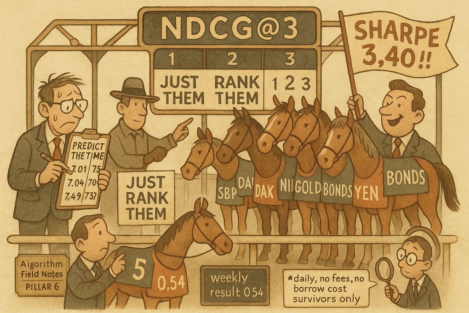
Cross-sectional momentum has one job: at each rebalance, order a universe of assets from worst to best, buy the top, sell the bottom. Everyone agrees on that. Where strategies quietly disagree is on how they produce the order. Classic momentum sorts on the past twelve-month return. A neural net predicts each asset's next return and sorts on the prediction. Both treat the ranking as a byproduct of something else, a raw return or a point forecast. But if the only thing you ever use is the order, why not train the model to get the order right directly?
That is the question this paper picks up, borrowing the answer from search engines. Information retrieval solved "put the most relevant thing on top" decades ago with learning-to-rank algorithms, and the paper drops one of them, LambdaMART, into a four-asset-class momentum backtest. The intellectual case is clean and it matches the old article "Ranking Beats Forecasting for Many Trading Problems": you should optimize the objective you actually trade on. The empirical case is where you need to keep your hand on your wallet. The headline number, a 3.40 Sharpe in equities, is a method demonstration, not a strategy, and the paper's own weekly results are what give the game away.
Four ways to build the same ordered list
Fix the portfolio first so the only thing that changes is the ranker. Every strategy scores each asset, sorts the scores, longs the top three, shorts the bottom three, equal-weights each leg, and scales positions so each asset contributes the same risk. The portfolio return on the day is the average of those signed, vol-scaled asset returns.
$$ r_{t,t+1}^{\text{CSM}} = \frac{1}{n} \sum_{i=1}^{n} S_t^{(i)} \, \frac{\sigma^{\text{tgt}}}{\sigma_t^{(i)}} \, r_{t,t+1}^{(i)}, \qquad S_t^{(i)} = \begin{cases} +1 & \text{rank} > N_t - 3 \\ -1 & \text{rank} \le 3 \\ 0 & \text{otherwise} \end{cases} $$
In words: the signal S is plus one for the three top-ranked assets, minus one for the three bottom-ranked, and zero for everyone in the middle. The ratio of target volatility to the asset's own volatility scales each position so a calm asset gets a bigger notional than a wild one, which is the same inverse-vol sizing behind the old article "Selection vs Diversification: Why |t|>3 Throws Away Alpha." Target vol is 15% annualized; each asset's vol is a 63-day exponentially weighted estimate.
Work one leg through it. Say the target is 15% annual (about 0.94% daily) and an equity index is running at 20% annual vol. Its scale factor is 15 divided by 20, so 0.75. If it is a top-three long and gains 1% that day, it contributes 0.75 times 1%, so 0.75%, to the long leg before averaging across the six positions. A 30%-vol index in the same slot gets scaled to 0.50 and contributes less. The sizing is fixed. The ranking is the only decision.
Now the four rankers. JT (Jegadeesh-Titman) scores each asset by its raw 252-day return and sorts. Baz scores by a blend of volatility-normalized MACD signals across three time scales, the CTA-style trend indicator. Both are hand-built formulas with no fitting. The two machine-learning rankers share the same 22 features per asset: the one-month raw return, volatility-normalized returns over 1, 3, 5, 10, and 21 days, and a stack of MACD indicators at different horizons.
Regress-then-rank: predict the return, sort the predictions
The multilayer perceptron is the honest strawman for "just forecast returns." It maps the feature vector to a number trained to match next day's volatility-scaled return under mean squared error, then you sort those numbers.
$$ L(\theta) = \frac{1}{M} \sum_{\Omega} \left( Y_t^{(i)} - \frac{r_{t,t+1}^{(i)}}{\sigma_t^{(i)}} \right)^2 $$
Read it as: average, over every asset-day in the training set, the squared gap between the model's score Y and the realized vol-scaled return. Minimizing this makes Y a good point forecast of return. The ranking is whatever falls out of sorting those forecasts.
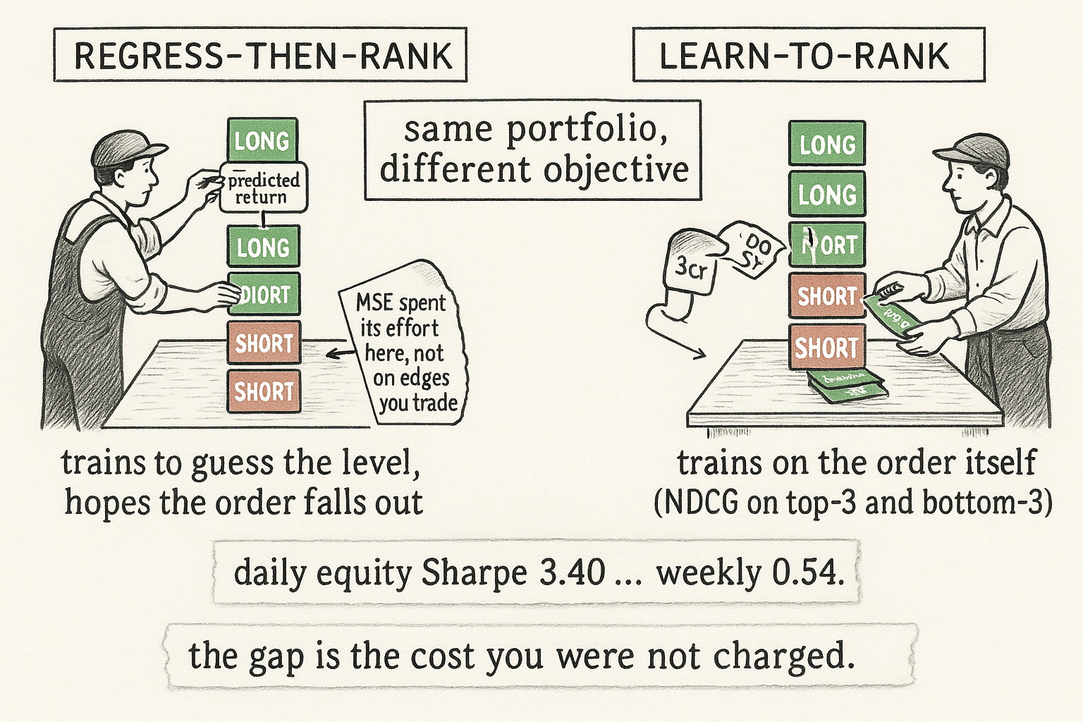
Here is the leak. MSE spends its effort where the errors are largest in magnitude, which is the middle of the pack and the fat tails, not the top and bottom edges you trade. Suppose two assets both belong in your short basket. The truth says asset A returns minus 2% and asset B minus 3%. A model that predicts minus 2.5% for both has real squared error but ranks them correctly enough for a top-3/bottom-3 trade. A second model nails A at minus 2% but calls B plus 1%. It has lower error on A yet flips B out of the short leg entirely. MSE cannot tell you the second mistake is the expensive one, because it grades forecast accuracy, not order. That mismatch between the loss and the objective is the whole opening for learning-to-rank.
Learn-to-rank: optimize the order you actually trade
LambdaMART attacks the order directly. It is a gradient-boosted tree ensemble descended from RankNet and LambdaRank, and instead of minimizing forecast error it optimizes a ranking-quality metric, NDCG, by defining gradients ("lambdas") that push assets toward their correct list positions.
$$ L(\theta) = \sum_{t \in \mathcal{T}} \ell\big(y_t^{(i)}, f(\mathbf{x}_t^{(i)}; \theta)\big)_{i \in \mathcal{U}}, \qquad \text{aggregated}_{\text{ndcg}} = \tfrac{1}{2}\big(\text{top}_{3,\text{ndcg}} + \text{bottom}_{3,\text{ndcg}}\big) $$
The left piece says the loss compares the true ordering y against the model's scores across the whole universe at each rebalance, not one asset at a time. The right piece is the scorecard: NDCG@3 measured on the top three, then again on the bottom three (by flipping the labels so "most negative" counts as "most relevant"), and averaged. NDCG rewards putting the right names in the right slots with more credit for getting the very top and very bottom right, using an exponential gain of two-to-the-relevance minus one. That exponential is also why the paper caps the universe near 31 assets, since larger relevance grades overflow a 32-bit integer in the ranking library.
A worked NDCG intuition. Your short basket should hold the three worst assets. If your model ranks them 1st, 2nd, and 4th worst, NDCG@3 is high but not perfect because one true bottom-3 name slipped to slot four and an impostor took its place. If it ranks them 1st, 5th, and 9th, NDCG@3 drops hard, because the discount for lower positions is steep and you are missing two of the three names that carry the leg. The metric grades exactly the thing the trade cares about, which MSE does not.
The training is walk-forward and disciplined: fit on a 5-year block, freeze the parameters, trade the next 5-year block, with a 90/10 train-validation split and early stopping. Data runs 2000 to 2023 across 16 commodities, 18 bond indices, 29 currencies, and 26 equity indices.
The equity result, and why it is a demo
In equity indices with daily rebalancing, the ranking framing looks decisive. LambdaMART posts a 3.40 Sharpe, the MLP 3.08, while sort-by-past-return (JT) sits at minus 1.88 and the CTA signal (Baz) at minus 0.25. Random ranking gives minus 0.11. The learners also cut max drawdown to minus 20% against JT's minus 100%, and lift the hit rate to 0.59.
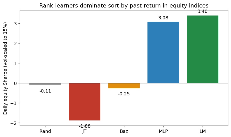
Before you wire up a broker, read the paper's own footnotes, because the author does not hide them. The equity results carry no transaction costs. The index universe comes from a screen that keeps major, actively traded indices, which is survivorship bias baked into the sample. Shorting indices is expensive and sometimes impossible, and daily rebalancing multiplies that cost. The author says it plainly: weekly performance is the more realistic indicator, and daily rebalancing "could significantly underestimate the transaction costs involved in shorting indices." A 3.40 Sharpe that assumes free, frictionless daily shorting of a curated index list is a statement about the algorithm, not about a tradable P&L.
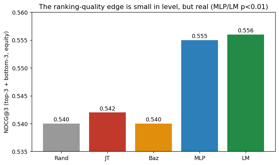
The ranking-quality edge that drives it is real but tiny in level. NDCG@3 in equities is 0.556 for LambdaMART and 0.555 for the MLP, against 0.540 for random, and both machine learners clear significance at the 1% level while JT (0.542) and Baz (0.540) do not. So the learners genuinely order equities better than a past-return sort does. The leverage from that small ranking gain to a 3.40 Sharpe is the part that only survives under frictionless daily rebalancing.
Slow the rebalance down and the story deflates
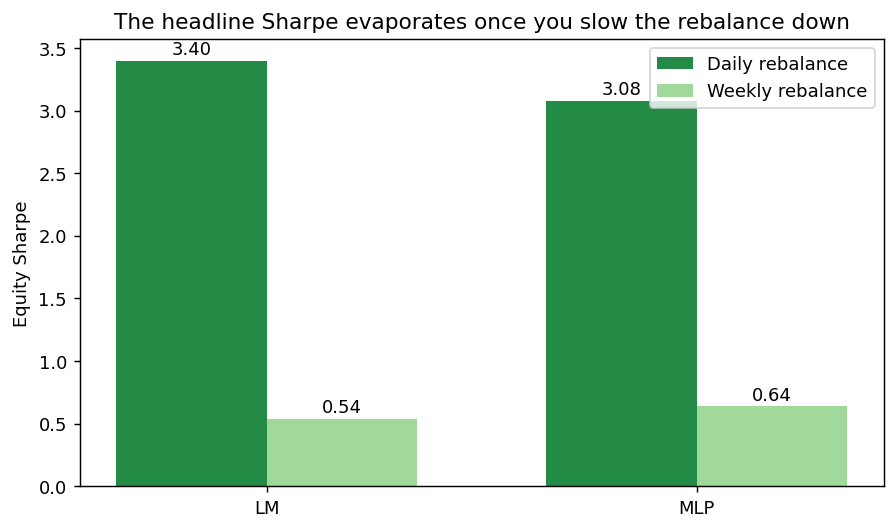
The cleanest test of whether the edge is tradable is to move to weekly rebalancing, where the author notes trading costs are negligible because only six positions turn over. If the daily Sharpe were a real signal rather than a rebalancing artifact, it should mostly survive. It does not.
Weekly equity Sharpe falls to 0.54 for LambdaMART and 0.64 for the MLP. The learners still beat the traditional strategies, which stay negative, so the ordering advantage is genuine and it persists. But the headline number drops by roughly a factor of six. Whatever produced 3.40 lived in the daily rebalance, exactly where costs are worst and least accounted for.
The author is candid about the mechanism: some cross-sectional signal decays at longer horizons, and the weekly sample is also thinner, which starves the learners of training data (35,211 daily training samples versus 6,786 weekly for currencies). Both cut the same way. The daily number is inflated by frictionless assumptions and possibly by overfitting a data-rich daily panel. Take 0.54, not 3.40, as the honest reading of what an equity learning-to-rank momentum strategy delivers, and even that ignores the survivorship bias in the index list.
Ranking structure is not universal
The paper's most useful finding for a practitioner is not the equity headline. It is that "momentum is a ranking problem" is true in some markets and false in others, which is why you cannot bolt LambdaMART onto everything and call it done.
| Asset class (daily) | Best ranker | LM Sharpe | MLP Sharpe | Best traditional | Read |
|---|---|---|---|---|---|
| Equity | LM | 3.40 | 3.08 | JT −1.88 | Ranking framing helps most, but demo-only |
| Bonds | MLP | 1.12 | 1.98 | JT 1.34 | Regress-then-rank wins; order matters less |
| Commodity | LM | 0.44 | 0.08 | JT −0.35 | LM the only consistent positive |
| Currency | LM | 0.47 | 0.00 | Baz 0.37 | Barely edges a hand-built signal |
In bonds the MLP's regress-then-rank approach beats LambdaMART, 1.98 to 1.12, and even simple JT momentum (1.34) beats the dedicated ranker. When you can forecast the level well, sorting the forecasts is fine and the ranking machinery adds nothing. In currencies the learner's 0.47 barely clears the hand-built Baz signal's 0.37, and weekly it gets worse: random ranking posts the best weekly currency Sharpe at 0.34 while LambdaMART manages 0.20. The author also strips out a hidden driver here, showing that the strong currency results in the prior literature were largely the Turkish Lira's collapse; excluding it pulls the numbers back to earth.
Two more cautions the paper surfaces. NDCG and Sharpe do not track each other cleanly, because in weekly currencies LambdaMART has the highest NDCG@3 yet no return edge, so better ranking on the metric does not guarantee better money. And random ranking scores NDCG@3 between 0.540 and 0.558 everywhere, which tells you the ranking task itself is hard and the achievable edge over a coin flip is thin. This is the same discipline the old article "Cross-Sectional Percentile Rank Within a Universe" insists on: a rank is only worth trading when the spread between top and bottom is real, not when the ordering is barely better than noise.
Where this lands
The idea is right and worth internalizing: if you only trade the order, train on the order. Learning-to-rank beats sort-by-past-return in equities and commodities on the metric that matters, and it does so with the same features a regress-then-rank model uses, which isolates the objective as the source of the gain. That is a real methodological upgrade over the reflex to forecast returns and sort them, and it extends the case the old article "Ranking Beats Forecasting for Many Trading Problems" makes at the single-instrument level to the cross-section.
What is not right is the headline. A 3.40 equity Sharpe assembled from frictionless daily shorting of a survivorship-screened index list is a benchmark for the algorithm, not a live edge, and the author's own weekly test collapses it to 0.54. Treat the daily equity number as a demo, treat the weekly number as the floor of what is real, and treat the cross-asset table as the actual lesson: ranking structure pays in equities and commodities, regress-then-rank is fine in bonds, and currencies barely beat noise. Match the tool to the market, and cost the trade before you believe the Sharpe.
KEY POINTS
- Cross-sectional momentum only uses the ordering of assets, so the sharpest framing is a ranking problem, not a return-forecasting problem. That is the paper's thesis and it matches "Ranking Beats Forecasting for Many Trading Problems."
- Regress-then-rank (an MLP under MSE) optimizes forecast accuracy, which spends effort in the middle and tails, not on the top-3/bottom-3 edges you actually trade. Learning-to-rank (LambdaMART) optimizes NDCG on those edges directly.
- With the portfolio and 22 features held fixed, the only variable is the ranker, so performance gaps isolate the objective.
- Daily equity Sharpe: LambdaMART 3.40, MLP 3.08, versus JT −1.88 and Baz −0.25. The ranking-quality edge is real but tiny in level (NDCG@3 0.556 vs 0.540 random, significant at 1%).
- The 3.40 is a method demo: no transaction costs, a survivorship-biased index universe, and expensive daily index shorting. Weekly rebalancing, where costs are negligible, drops it to 0.54.
- Ranking structure is not universal. Bonds prefer regress-then-rank (MLP 1.98 > LM 1.12 > JT 1.34), currencies barely beat a hand-built signal, and weekly random ranking wins in currencies.
- NDCG and Sharpe do not move together, and random ranking scores 0.540 to 0.558 everywhere, so the achievable ordering edge over noise is thin. Only trade a rank when the top-to-bottom spread is real.
A note on AI. The ideas, research, analysis, and conclusions in this article are my own. I use AI tools to help with editing and wordsmithing, because English is not my first language, and I am not shy about that. AI-generated ideas and AI-assisted writing are not the same thing: the first is empty slop from a generic prompt, the second is a tool for communicating years of real research more clearly. Judge the work by its substance, not by whether software helped polish the prose.