7. Python Research Notebooks November 22, 2026 13 min

7.7 The Vice of Complexity: Four Times the Simple Model Won

Equity premium timing: leave the intercept unpenalized and a 15-predictor ridge beats 12,000 features. On short samples the small fit wins.

Kelly, Malamud and Zhou's market-timing book trains 12,000 random features on 12 months of the CRSP value-weighted excess return, scaled by a trailing 12-month volatility, and bets that forecast as the position. They argued the out-of-sample Sharpe ratio rises with the feature count. Daniel Buncic re-estimated the same book on the January 1940 to December 2020 window, and the advertised complex specification earns a Sharpe ratio of 0.49. Forcing the regression through the origin, on a target with a positive mean, produces that rise. Short samples show up again in a Bitcoin close forecast, a fair-value filter, and a limit-order classifier, and the small fit is the one that survives the window in front of you.

Complexity is the feature count divided by the window

Complexity, written c, is the number of features P divided by the number of training months T.

$$ c = \frac{P}{T} $$

P of 12,000 on T of 12 is a complexity of 1,000. The specification that wins on the long window, once an intercept is allowed, uses 200 features and 120 months, so c is 200 divided by 120, which is 5/3. Lengthening the window lowers complexity even if you keep every feature. A higher Sharpe ratio at a longer window is a higher Sharpe ratio at a lower c.

Those 12,000 features are not 12,000 new facts. The information set is 15 monthly equity-premium predictors. A random Fourier feature draws a 15-by-1 weight, omega, from a standard normal, takes its dot product with the predictor vector G, scales by gamma (set to 2), and stores a sine and a cosine.

$$ S_{i,t} = \begin{bmatrix} \sin(\gamma \, \omega_i' G_t) \\ \cos(\gamma \, \omega_i' G_t) \end{bmatrix} $$

Worked toy on two coordinates, invented so the arithmetic is visible. Let G be (0.1, minus 0.2) and omega be (1, 0). The dot product is 0.1. Times gamma of 2 that is 0.2. Sine of 0.2 is 0.1987. Cosine of 0.2 is 0.9801. That pair is one draw. Another omega builds another pair from the same G. The parameter count grew. The information set did not.

Fit by ridge. Buncic's shrinkage z is added to the diagonal of the feature second-moment matrix. Shen and Xiu's lambda is a different penalty on a different scale.

$$ \hat{\beta}(z) = \left( z I + \frac{1}{T} \sum_{t=1}^{T} S_t S_t' \right)^{-1} \frac{1}{T} \sum_{t=1}^{T} S_t R_{t+1} $$

The inverted term is the feature second-moment matrix with z on the diagonal. The other term is the covariance between the features and next month's scaled return. One feature, so both are scalars. Suppose the feature's mean square is 1 and its covariance with next month's scaled return is 0.15. At z of 0 the coefficient is 0.15. At z of 6 it is 0.15 divided by 7, which is 0.0214. At z of 1,000 it is 0.15 divided by 1,001, which is 0.00015. A z of 1,000 on a 15-predictor benchmark wipes the slopes.

The position is the forecast. The timing return is that forecast times the realized scaled excess return.

$$ \pi_t = \hat{R}_{t+1|t}, \qquad R^{\pi}_{t+1} = \pi_t \, R_{t+1} $$

A forecast of plus 0.20 against a realization of plus 0.80 pays 0.16, in units of trailing volatility, not dollars. A negative forecast times a negative realization pays the same way, because the product of two negatives is positive. You are long or short by the size of the prediction.

The target's sample mean is 0.1590 in those volatility units. Buncic prints a robust standard error of 0.0336 and a t-statistic of 4.47. Divide 0.1590 by 0.0336 and you get 4.73, not 4.47, so one of those three printed figures does not match the other two. The source may have rounded a standard error it did not show. The direction is clear either way: the mean sits several standard errors above zero, and none of the 15 predictors has a zero mean either. Force the fit through the origin and the slopes have to manufacture that mean out of regressors that are themselves off zero. For the headline 12,000-feature model, squared forecast bias runs from 0.0130 to 0.0267 with the intercept shut, and falls below 0.0002 once the intercept is estimated and left out of the penalty. Taking 0.0002 as the ceiling, 0.0130 divided by 0.0002 is 65, and the restricted bias is higher than that ceiling, so the drop is more than 65-fold at the low end of the range.

The old article "Does Complexity Actually Help? The Virtue-of-Complexity Autopsy" takes apart the other choice in the same design. Buncic draws 1,000 sets of random features. Averaging the 1,000 forecasts and then scoring that one book is a portfolio you could hold. Scoring each draw and averaging the 1,000 Sharpe ratios is a different object. Expected return is linear, so the two routes agree on it. The Sharpe ratio is nonlinear, and the per-draw average traces a rising curve on a strategy whose content does not change with P. The pooled forecast is the book you would trade.

Shrink a weak coefficient; do not delete it

Shen and Xiu define a weak signal as a slope vector whose squared length vanishes while the predictor count grows.

$$ \| \beta_0 \|_2^2 \asymp_P \tau \to 0, \qquad p \to \infty $$

Beta-zero here is the vector of true slopes, tau is that shrinking budget, and p is the predictor count. Population R-squared moves with tau. A population R-squared of 1 percent means the true slopes explain one part in a hundred of the variance of the outcome. In that regime the zero estimator, which forecasts 0 on every row and ignores every column, matches the Bayes predictor that knows the prior, to first order. Clearing zero is the evidence that a method learned something.

Ridge, lasso, and zero all reach that first-order risk, so a risk ratio near 1 cannot separate them. The gap worth looking at is a magnified prediction error.

$$ \Delta(\hat{\beta}) = p \, n^{-1} \, \tau^{-2} \left( \| \Sigma_2^{1/2} (\hat{\beta} - \beta_0) \|^2 - \| \Sigma_2^{1/2} \beta_0 \|^2 \right) $$

The parentheses hold your estimator's prediction error minus the zero estimator's prediction error. The factor in front, p over n times 1 over tau-squared, rescales a small difference into a limit you can sign. Negative means the estimator beats a forecast of zero. Positive means the zero forecast had the lower error.

For ridge, with the tuning parameter written as lambda over tau, the limit is closed form.

$$ \Delta(\hat{\beta}_r) \xrightarrow{P} \alpha^{*} = 2 \theta_2 \sigma_x^{4} \left( \frac{\sigma_{\varepsilon}^{2} \theta_1}{2 \lambda^{2}} - \frac{\sigma_{\beta}^{2}}{\lambda} \right) $$

Set theta-two, sigma-x, sigma-epsilon, theta-one, and sigma-beta all to 1. The 2 and the 1/2 cancel, and alpha-star equals 1 over lambda-squared, minus 2 over lambda. At lambda of 1 that is 1 minus 2, so minus 1: ridge sits one unit below the zero forecast, and that is the bottom of this curve. At lambda of 2 it is 0.25 minus 1, so minus 0.75, still below zero. Send lambda to infinity and alpha-star returns to zero from below, because a huge penalty is the zero forecast. Send lambda toward 0 and alpha-star runs to positive infinity. The ridgeless fit, the minimum-length interpolator that passes through every training point, then loses to a forecast of zero. The lambda that minimizes the expression is sigma-epsilon-squared times theta-one, divided by sigma-beta-squared. Under these constants that lambda is 1, and plugging it back in returns minus 1. The formula and the optimum agree.

Lasso has no closed form in their argument. They bound the magnified error instead, and both the lower and the upper bound stay non-negative at every penalty. A large penalty turns lasso into the zero forecast. A small penalty sends the error to positive infinity. Selection wants a hard split between real predictors and noise. Weak signals remove the split, and a coefficient set exactly to zero drops a slice of a diffuse sum that ridge would have shrunk and kept. The old article "Can Machines Learn Weak Signals? Ridge > Zero > Lasso" is the six-dataset grid this bound was written to explain. Cross-validation still picks a ridge penalty on the useful part of the curve when tau is unknown.

A rejected order is already a forecast

On the Hyperliquid BTC-USD perpetual, a post-only buy that would cross the spread is rejected on arrival. It never rests in the book, never prints in the ordinary market-data feed, and cannot move the mid. Albers, Cucuringu, Howison, and Shestopaloff regress the next 10-second midprice return, in basis points, on the sign of that rejection.

$$ R_t = \beta_0 + \beta_1 \, 1_t^{\mathrm{rej}} + \varepsilon_t $$

In this regression, beta-zero is the intercept. The indicator equals plus 1 for a rejected buy and minus 1 for a rejected sell. The fitted intercept is minus 0.1178, the slope is 0.4242, both with a standard error of 0.0003, and the R-squared is 0.022. A rejected buy lines up with minus 0.1178 plus 0.4242, which is 0.3064 basis points over the next ten seconds. A rejected sell lines up with minus 0.1178 minus 0.4242, which is minus 0.5420. The sign of the order that never landed matches the direction of the next price change 72.3 percent of the time.

The rejected-flow imbalance over the last 100 post-only submissions has the same shape as a top-of-book imbalance.

$$ \mathrm{imb}_t^{\mathrm{rej}} = \frac{V_{t,\mathrm{buy}}^{\mathrm{rej}} - V_{t,\mathrm{sell}}^{\mathrm{rej}}}{V_{t,\mathrm{buy}}^{\mathrm{rej}} + V_{t,\mathrm{sell}}^{\mathrm{rej}}} $$

Seventy units of rejected buy volume and thirty of rejected sell volume give (70 minus 30) over 100, which is 0.40. In the regression that puts this imbalance next to the single-order sign, the imbalance coefficient is 0.5415 and the single-order slope falls from 0.4242 to 0.1354. The R-squared moves from 0.022 to 0.033. The single rejection is a draw from the flow.

The comparative regression adds the visible book: top-of-book imbalance, the spread after subtracting the daily mean and dividing by the daily standard deviation, the rejected-flow imbalance, and the imbalance of post-only orders that were accepted.

$$ R_t = \beta_0 + \beta_1 \, \mathrm{imb}_t + \beta_2 \, \mathrm{Spread}_t + \beta_3 \, \mathrm{imb}_t^{\mathrm{rej}} + \beta_4 \, \mathrm{imb}_t^{\mathrm{open}} + \varepsilon_t $$

The fitted values are an intercept of minus 0.1366, a book-imbalance slope of 0.6224, a spread slope of 0.0305, a rejected-imbalance slope of 0.1674, and an accepted-order slope of 0.0705. The R-squared is 0.045. The rejected-flow slope divided by the accepted-flow slope is 0.1674 divided by 0.0705, which is 2.37. Set all three imbalances to plus 1 and the standardized spread to 0. The fitted return is minus 0.1366 plus 0.6224 plus 0.1674 plus 0.0705, which is 0.7237 basis points. The paper calls a forecast of this kind "at most a few tenths of a basis point." That wording matches the univariate 0.31 basis points. It sits low relative to the stacked sum, which is 0.72. Both sit under the taker fee of 1.44 to 2.7 basis points. The one-bit regression's R-squared of 0.022 is 0.022 divided by 0.045, or 0.49, of the four-variable R-squared.

The sample is September 2025, one month. Rejected post-only submissions run at about 60,310 a minute, about 86 percent of order submissions, on the order of 3.3 billion dollars of notional a minute. The rejection feed arrives with enough extra delay that this ten-second regression is a research result, not a live order.

The smaller specification wins four times

The right-hand bar in each panel is the smaller specification. On the Bitcoin panel a shorter bar is a tighter error.

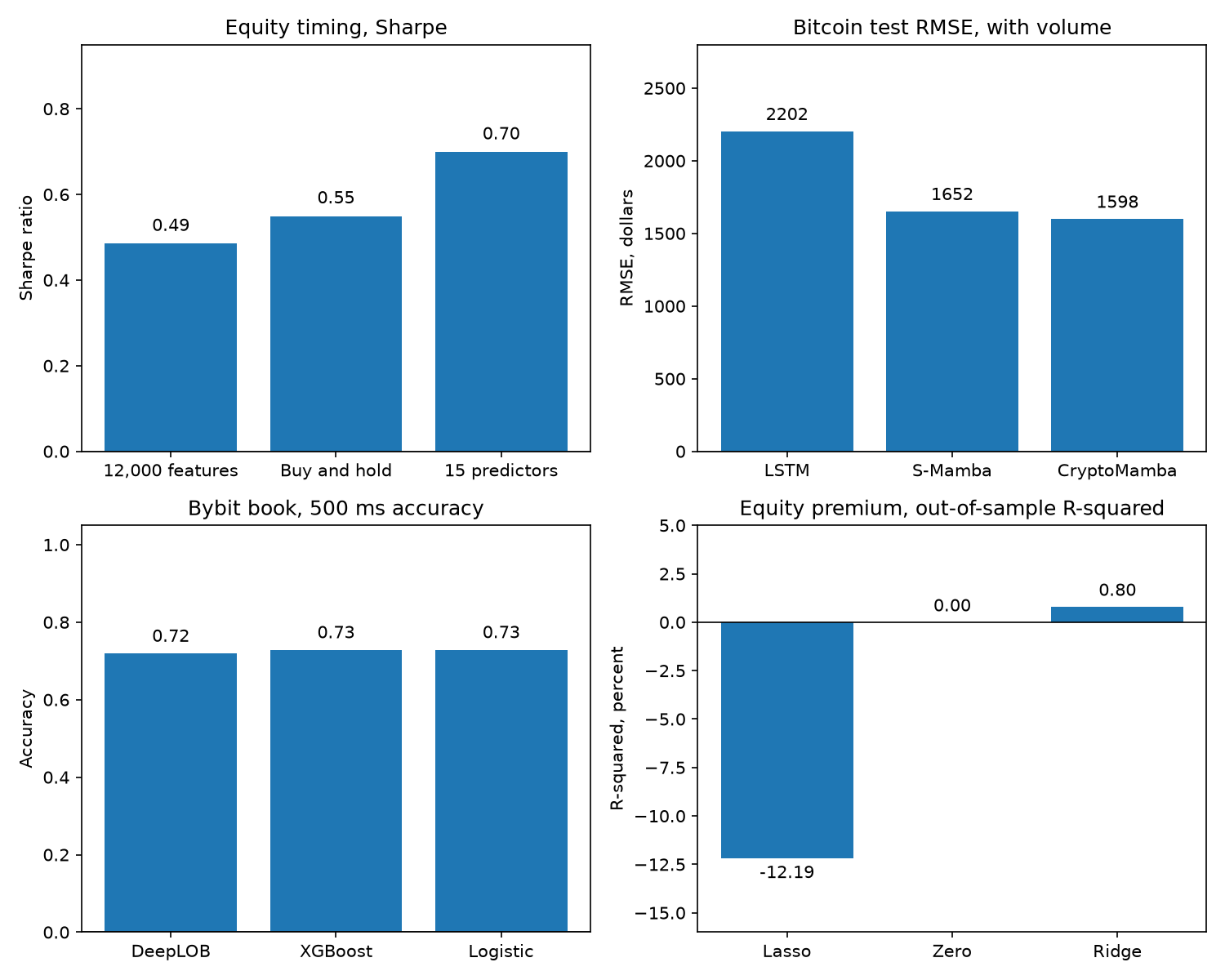
Four panels of smaller versus larger specifications. Equity-timing Sharpe ratios of 0.49, 0.55, and 0.70. Bitcoin test RMSE of 2202, 1652, and 1598 dollars. Bybit 500-millisecond accuracies of 0.72, 0.73, and 0.73. Annual equity-premium out-of-sample R-squared of minus 12.19 percent, zero, and plus 0.80 percent.

On the equity-timing panel that bar is 0.70, against 0.49 for the 12,000-feature book and 0.55 for buy-and-hold on the same volatility-scaled series. Those are 0.6990, 0.4851, and 0.5494 before rounding. The 0.70 is the best expanding-window ridge on the 15 predictors across Buncic's shrinkage grid, at z of 0.4 and T of 120. The 0.49 is one pre-specified book: 12,000 features, z of 1,000, intercept shut.

CryptoMamba's volume-on test RMSE is 1598.1 against 1651.6 for S-Mamba and 2202.1 for an LSTM; logistic regression on the 500-millisecond, 40-level Bybit book scores 0.7284 against DeepLOB at 0.7189, while a separate one-second depth cut takes XGBoost from 0.7150 at 40 levels on 5,442 test rows to 0.5797 at 5 levels on 18,336 rows; ridge on the annual equity premium, 16 predictors, posts an out-of-sample R-squared of 0.80 percent against lasso at minus 12.19 percent and ordinary least squares at minus 81.08 percent; and the old article "Fair Value as an Adaptive Low-Pass Filter: LAFO for Mean Reversion" records a two-layer net at an in-sample Sharpe ratio of 11.05 against WaveNet at 8.01 and a deep Kalman filter at 4.92.

Read the gaps off those figures before you rank architectures. On the Bitcoin panel, 1651.6 minus 1598.1 is 53.5 dollars of RMSE, 3.2 percent of the S-Mamba error, on one year of daily bars. On the validation year, the volume-inclusive LSTM finishes ahead of CryptoMamba on the extended-smart rule, and the test year reverses that order. On the book panel, 0.7150 minus 0.5797 is 0.135 of accuracy when the depth cut also changes the test set, while 0.7284 minus 0.7189 is 0.0095 between logistic regression and DeepLOB on the row where both see 40 levels. The equity-premium ordinary-least-squares figure, minus 81.08 percent, comes from a training sample that bottoms out at 17 annual observations against 16 predictors. The fair-value 11.05 is in-sample.

Run the small model before you add a layer

Divide P by the window you will refit. A complexity above 1 means the fit is already a regularized one, and the writeup should say which penalty did the regularizing.

Refit with an intercept and leave the intercept out of the penalty. If the curve that rose with P flattens, the intercept was carrying it. The old autopsy is the full account of the averaged-Sharpe version of that curve. This check is the one you can run on a single pooled book in an afternoon.

When the out-of-sample R-squared in the market you trade is a few percent, fit ridge, fit a zero forecast, and only then fit lasso. Shen and Xiu show that cross-validation still lands on the useful part of the ridge curve when the signal budget tau is unknown. Lasso's bounds stay non-negative in that region. A sparse screen is the wrong first tool there.

On a limit-order book, compute the top-of-book imbalance, and the signed rejection if the feed has it, and score a logistic regression before you add a convolutional layer. That 0.73 is an offline score. Wang's Savitzky-Golay smooth is a centered cubic on 21 snapshots, and at a 100-millisecond clock the ten snapshots on the right of that window are the next second of prices. The old article "Better Inputs Beat Deeper Nets: Crypto LOB Direction" already compares that smooth with a filter that only looks backward. The file is one day, 2025-01-30, and any row missing the depth you asked for is dropped, which is why 40 levels leaves 5,442 test rows and 5 levels leaves 18,336.

Price the fitted return against the fee you will pay. A rejected-buy forecast of 0.31 basis points, or 0.72 if every imbalance in the comparative regression is pushed to plus 1, sits under a taker fee of 1.44 basis points. The old article "State-Space Models for Price: CryptoMamba vs Transformers (Skeptical)" makes the matching point on the daily Bitcoin book: the level of a near-random-walk is an easy regression target, and one year with one random seed leaves a 136,000-parameter state-space net within a few percent of RMSE of the next model.

I am against adding a hidden layer, a random-feature expansion, or a lasso screen until the small model, with an unpenalized intercept, has lost on a window you did not use to crown it. The timing book resizes every month off a short refit, and Buncic's comparison charges no spread. The predictor set uses contemporaneous inflation, which is released about two weeks into the following month, and replacing it with lagged inflation lowers the random-feature Sharpe ratios for every feature count and every z. The fair-value Sharpe is a methodological demo on two months of 2-minute bars. Read each panel in its own unit. None of these panels is a sizing input.

KEY POINTS

Divide feature count by the training window before you add a feature. Twelve thousand features on twelve months is a complexity of 1,000.
Leave the intercept out of the penalty. The 15-predictor expanding ridge then posts a Sharpe ratio of 0.70 on the 1940 to 2020 window.
Shrink weak predictors with ridge. On the annual equity premium, lasso posts an out-of-sample R-squared of minus 12.19 percent.
Score logistic regression on the book before you add a convolutional layer. On the 500-millisecond Bybit sample that accuracy is 0.73.
Price a rejected-buy forecast against the fee before you treat it as impact. The univariate fit is 0.31 basis points over ten seconds.

References

A note on AI. The ideas, research, analysis, and conclusions in this article are my own. I use AI tools to help with editing and wordsmithing, because English is not my first language, and I am not shy about that. AI-generated ideas and AI-assisted writing are not the same thing: the first is empty slop from a generic prompt, the second is a tool for communicating years of real research more clearly. Judge the work by its substance, not by whether software helped polish the prose.