10.17 Can Machines Learn Weak Signals? Ridge > Zero > Lasso

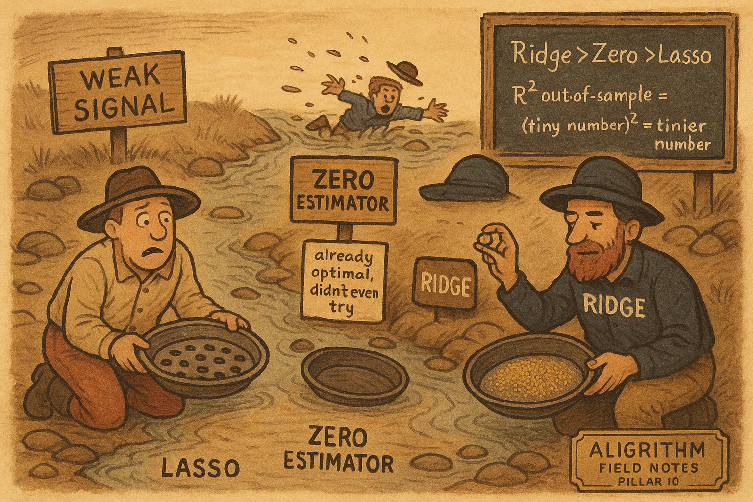
Feed 920 firm characteristics into a Lasso to predict next month's stock returns and it will do something that should stop you cold: it loses to a model that predicts zero for every stock. Not "underperforms a good benchmark." Loses to the number 0. Shen and Xiu prove this is not bad luck or a coding bug. In the regime where economics and finance actually live, where signals are individually tiny and predictors are plentiful, Lasso cannot beat the zero estimator for any choice of its penalty, while Ridge can. The ranking is Ridge, then zero, then Lasso, and it holds in theory and across six real datasets.

Start with why the regime matters. The authors hand-collected the R-squared from every regression in 411 economics papers and 380 finance papers published in 2022, more than 20,000 values. The 25% quantile sits at 9.7% for economics and 5.8% for finance, and that is after publication bias filters out the weakest results. Most published work in these fields runs on covariates with feeble explanatory power.

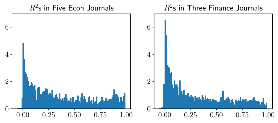
That concentration near zero is the whole setup. When no single predictor carries much signal, the useful question stops being "which model fits best" and becomes "can any model beat doing nothing at all." The old article "Does ML Actually Help Asset Pricing? Kelly's 20%, Not 2-3x" landed on a modest verdict for machine learning in the cross-section; this paper explains the mechanism underneath that modesty and tells you which regularizer to reach for when the signal is this thin.

The zero estimator, and why it is the bar to clear

A weak signal is a coefficient so small its estimation error swallows the bias it would remove. Formally the paper defines the weak regime by the total signal strength vanishing as the number of predictors grows.

$$ \| \beta_0 \|_2^2 \asymp_P \tau \to 0, \qquad p \to \infty $$

Read it plainly: beta-zero is the vector of true coefficients, and the squared length of that vector, its total signal energy, shrinks toward zero (call that shrinking budget tau) while the number of predictors p grows without bound. The population R-squared is proportional to tau, so tau near zero means an R-squared near zero. Worked example: if tau delivers a population R-squared of 1%, then even the true coefficients explain one part in a hundred of return variance. There is almost nothing to learn, and the question is whether a method can extract even that.

The natural benchmark in this world is the zero estimator, which ignores every predictor and forecasts zero. It sounds like a strawman. It is not. Shen and Xiu prove that when signals are this weak, the zero estimator is asymptotically Bayes-optimal: its prediction risk matches the best possible predictor that knows the true prior distribution of the coefficients.

$$ \lim_{n \to \infty} \frac{\mathcal{R}(\hat{\beta}, F)}{\mathcal{R}(F)} = 1 \quad\text{for } \hat{\beta} = 0 $$

The numerator is the risk of the estimator you built; the denominator is the risk of the infeasible Bayes predictor. When that ratio goes to 1, your estimator is doing as well as anything possibly could. The theorem says the do-nothing forecast hits that mark. So beating zero is not a low bar you clear by accident. Beating zero means you genuinely pulled signal out of the noise, because zero is already optimal to first order. Any estimator that fails to beat it has learned nothing.

The test that magnifies the difference

Because Ridge, Lasso, and zero all hit the same first-order optimal risk, comparing their risk ratios tells you nothing; they all look like 1. To separate them you need a microscope. The paper defines a relative-error metric that blows up the higher-order gap and carries a sign.

$$ \Delta(\hat{\beta}) = p\, n^{-1} \tau^{-2} \left( \| \Sigma_2^{1/2}(\hat{\beta} - \beta_0) \|^2 - \| \Sigma_2^{1/2} \beta_0 \|^2 \right) $$

The bracket is the estimator's prediction error minus the zero estimator's prediction error (the zero estimator's error is just the second norm, since it sets beta-hat to zero). Multiply by p over n times tau-squared-inverse to rescale the tiny difference into something that converges to a finite number. The sign is what matters: if Delta is negative with probability approaching one, your estimator beats zero; if positive, it loses to zero. Worked reading: Delta equal to -1 means you edged out the do-nothing forecast; Delta equal to +2 means you would have been better off forecasting zero and going home.

Ridge dips below the line; Lasso never does

Run Ridge through this metric and the payoff is a clean closed form. With the tuning parameter written as lambda over tau, the relative error converges to a value the paper calls alpha-star.

$$ \Delta(\hat{\beta}_r) \xrightarrow{P} \alpha^* = 2\theta_2 \sigma_x^4 \left( \frac{\sigma_\varepsilon^2 \theta_1}{2\lambda^2} - \frac{\sigma_\beta^2}{\lambda} \right) $$

The term in parentheses is a parabola in one-over-lambda: a positive piece that dies like lambda-squared and a negative piece that dies like lambda. Set the noise, signal, and design constants all to one and it collapses to alpha-star equal to one-over-lambda-squared minus two-over-lambda. Plug in numbers. At lambda equal to 1, alpha-star is 1 minus 2, so -1: Ridge beats zero by the most. At lambda equal to 2, it is 0.25 minus 1, so -0.75, still negative. As lambda grows the curve creeps back up toward zero from below, meaning Ridge with a huge penalty just becomes the zero estimator and ties it. Push lambda toward zero and alpha-star runs to positive infinity: the Ridgeless (no-penalty) interpolator is catastrophically worse than doing nothing, because with weak signals its implicit regularization cannot control variance and the fitted coefficients balloon far past the true ones.

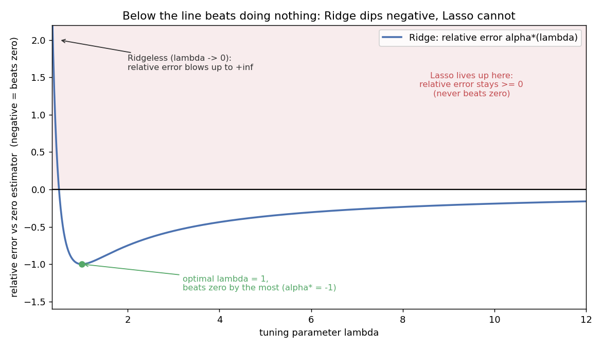
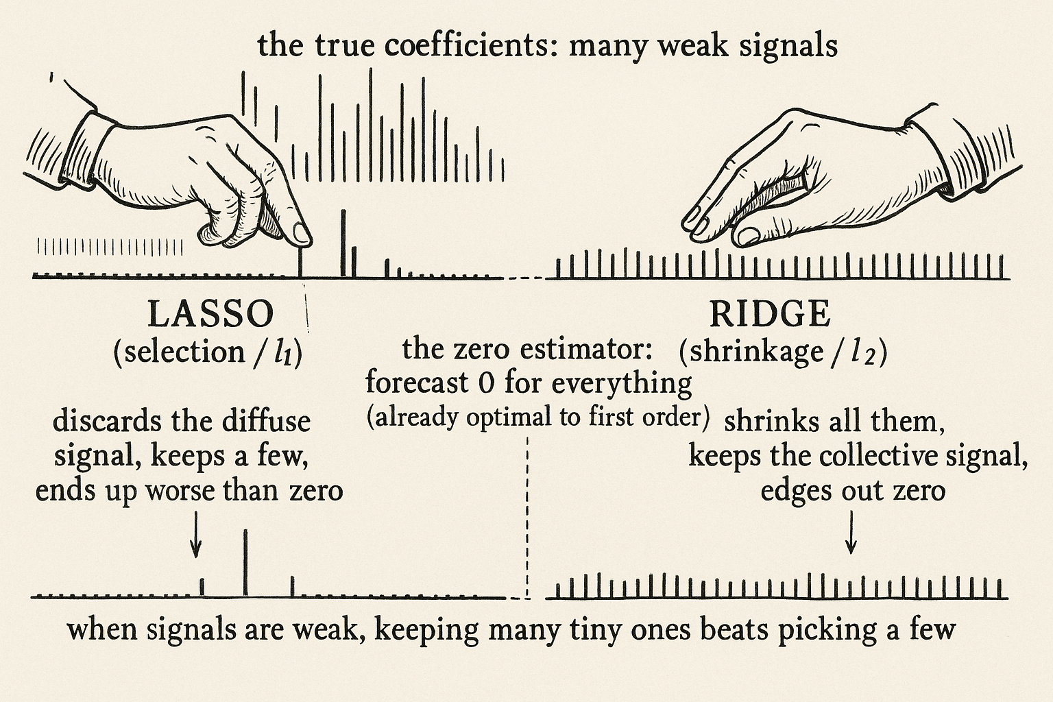
Now Lasso. The paper cannot get a closed form because Lasso has no closed-form solution, so it derives probability bounds instead, and the bounds are the punchline: both the lower and upper bounds on Lasso's relative error are non-negative, for every choice of the penalty. Lasso lives in the shaded region above the zero line in the chart and cannot cross it. Crank its penalty up and it converges down to zero (it becomes the zero estimator); crank it down and it diverges to positive infinity (worse than zero). There is no setting where it dips negative. The reason is structural. Lasso is a selection method that thrives when there is a crisp line between real and fake predictors. Weak signals erase that line, so Lasso's willingness to zero out coefficients throws away exactly the diffuse, collective signal that Ridge's shrinkage keeps. The elastic net inherits the problem to the extent it leans on the l1 penalty.

One practical rescue: cross-validation still works for Ridge here. Even though the optimal penalty diverges as the sample grows (because tau is unknown and shrinking), the K-fold cross-validated choice converges to the noise-to-signal ratio and lands you on the useful part of the curve without knowing tau in advance.

Six datasets say the same thing

Theory is cheap. Shen and Xiu run seven methods across six datasets from finance, macro, and micro. The pattern from Table 1 is stubborn.

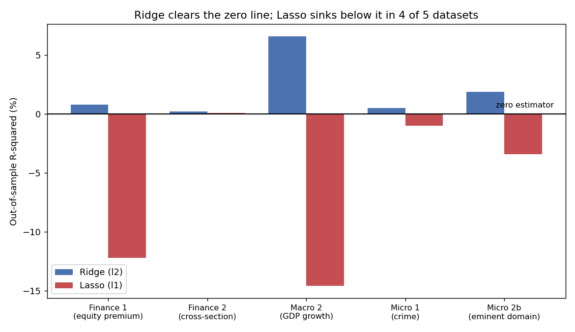
Predicting the equity premium from the Welch-Goyal indicators (16 predictors, annual data since 1948), Ridge posts an out-of-sample R-squared of 0.80% while Lasso posts -12.19%, and plain OLS, with barely more observations than predictors, craters to -81.08%. On the Gu-Kelly-Xiu cross-section of individual stock returns, extended with 920 characteristics, the l2-penalized neural net leads at 0.26% and Ridge follows at 0.19%, both beating the l1 neural net at 0.14% and Lasso at 0.10%. Turn those thin R-squared numbers into a long-short decile portfolio and the l2 neural net earns a Sharpe of 2.13 and Ridge 1.64, while the sparse GBRT trails at 0.80. Cross-country GDP growth: Ridge 6.58%, Lasso -14.58%. Crime rates: Ridge 0.48%, Lasso -1.01%. Only one of the five low-signal cases has Lasso clearing zero at all.

The pairing extends past linear models. Random Forest, which builds dense trees using nearly all variables, beats Gradient Boosting, which builds sparse sequential trees, in every weak-signal dataset. Neural nets with an l2 penalty beat the same nets with an l1 penalty. Across the board, the denser method wins. Look at the variable-importance plots and the winners spread small weights across almost every covariate; the losers concentrate on a handful. That is the collective-signal story made visible.

Signal weakness, not the absence of sparsity

Here is where the paper picks a fight with a famous result. Giannone, Lenza, and Primiceri argued that sparsity is an "illusion" in economics: the best predictive models keep lots of covariates, so the world is not really sparse. Shen and Xiu accept the empirics and reinterpret the cause. Ridge can beat Lasso even when the true model is genuinely sparse, as long as the non-zero coefficients are weak. So Lasso's failure does not prove the world is dense. It proves the signals are weak. Watching Lasso underperform tells you about signal strength, not about the number of true predictors.

This reframes the old article "The Factor Zoo and the Multiple-Testing Reckoning" from the shrinkage side. That piece, through the Kozak-Nagel-Santosh lens, argued the cross-section is better described by a dense stochastic discount factor than by a few clean anomalies, and that shrinking many weak factors beats selecting a few strong ones. This paper supplies the estimation-theory reason: when factors are individually weak, an l2 shrinker that keeps all of them is asymptotically the right tool, and an l1 selector that discards most of them is asymptotically the wrong one. The debate about whether alpha is sparse or dense partly dissolves into a debate about whether the signals are strong or weak, and in asset pricing they are weak.

What survives when signals are weak

The proposition on out-of-sample R-squared drives home how thin the payoff is even when you win.

$$ R^2_{oos}\big(\hat{\beta}_r(\lambda_n^{opt})\big) = \frac{n}{p}\, \theta_2 \, (R^2)^2 \,\big(1 + o_P(1)\big) $$

The optimal Ridge's out-of-sample R-squared is proportional to the square of the population R-squared, scaled by the sample-to-predictor ratio n over p. Square a small number and it gets much smaller. Worked example: population R-squared of 5% (0.05), with n over p times theta-2 near one, gives an out-of-sample R-squared around 0.05 squared, so about 0.25%. The signal is real, Ridge captures it, and the visible out-of-sample R-squared is still a quarter of a percent. That is not a bug in your pipeline. It is what learning a weak signal looks like, and it is exactly why the Sharpe ratios above come from R-squared values you could mistake for zero.

The trap the old article "Does Complexity Actually Help? The Virtue-of-Complexity Autopsy" warned about sits right next to this result. Complexity and flexibility are not free in a low-signal world: the Ridgeless interpolator, the most complex linear fit, is the one that blows up worst here, and the shallow neural nets can lose to plain Ridge because their extra parameters chase noise. Flexible models help only after you have shrunk hard, and shrinkage with an l2 penalty is doing most of the work.

Where this connects

The spine of this pillar is the equation from the old article "What a Factor Actually Is: alpha + beta-lambda, and Why the Market Is Factor #1," where the cross-section of expected returns is a set of weak, noisy loadings on priced factors. This paper is the estimation manual for that world. When the true premia are small and the characteristics are many, ridge-style shrinkage of the whole coefficient vector beats lasso-style selection, boosting-style sparse trees, and unregularized fits, and the honest out-of-sample R-squared you should expect is the square of an already small number.

The practical takeaways are blunt. Benchmark against the zero estimator, not against a flattering baseline, because zero is the optimal do-nothing forecast when signals are weak. Prefer l2 penalties (Ridge, l2 neural nets, Random Forest) over l1 penalties (Lasso, GBRT) in these regimes. Read a low out-of-sample R-squared as evidence of weak signal, not proof of a sparse world. And treat Lasso's popularity as a modern OLS with suspicion: in economics and finance, where the R-squared histograms pile up near zero, it is the wrong default.

KEY POINTS

• In the high-dimensional, low-R-squared regime that describes most of economics and finance (25% quantile R-squared of 9.7% and 5.8%), the zero estimator is asymptotically Bayes-optimal. Beating it means you genuinely learned a weak signal.
• Ridge can beat the zero estimator with the right l2 penalty; its relative error dips negative, bottoming out at the optimal tuning value. Lasso cannot beat zero for any l1 penalty, because its relative-error bounds are provably non-negative.
• The Ridgeless (no-penalty) interpolator is worse than doing nothing in this regime; its implicit regularization fails to control variance and the fitted coefficients balloon.
• The ranking generalizes: dense Random Forest beats sparse Gradient Boosting, and l2 neural nets beat l1 neural nets, in every weak-signal dataset. Denser methods win because weak signal is spread across many predictors.
• Six real datasets confirm it. Equity premium: Ridge 0.80% versus Lasso -12.19%. Cross-section of returns: l2 neural net Sharpe 2.13, Ridge 1.64, sparse GBRT 0.80. Ridge clears zero in all five low-signal cases; Lasso clears it in one.
• Lasso failing does not prove the model is dense. Ridge beats Lasso even under true sparsity if the non-zero coefficients are weak. The binding constraint is signal weakness, not the absence of sparsity.
• Even when Ridge wins, out-of-sample R-squared is proportional to the square of the population R-squared, so a 5% population R-squared shows up as roughly 0.25% out of sample. Cross-validation still selects a valid Ridge penalty without knowing the signal strength.

References

• Economic Predictions With Big Data: The Illusion of Sparsity (Giannone, Lenza, and Primiceri, 2021)
• Empirical Asset Pricing via Machine Learning (Gu, Kelly, and Xiu, 2020)
• Ridge Regression: Biased Estimation for Nonorthogonal Problems (Hoerl and Kennard, 1970)
• Regression Shrinkage and Selection via the Lasso (Tibshirani, 1996)
• Regularization and Variable Selection via the Elastic Net (Zou and Hastie, 2005)
• The Lasso Risk for Gaussian Matrices (Bayati and Montanari, 2012)
• A Comprehensive Review of Prediction of Stock Returns via the Equity Premium (Welch and Goyal, 2008)
• Shrinking the Cross-Section (Kozak, Nagel, and Santosh, 2020)
• Can Machines Learn Weak Signals? (Shen and Xiu, 2024)