10.16 ML in the Cross Section: Avramov's Companion to the DDA3600 Spine
Neural-net cross-section alpha dies once you drop microcaps and charge 0.50% of turnover: FF6 0.31% vs cost 0.43%. Linear IPCA still clears, 0.61% vs 0.57%.
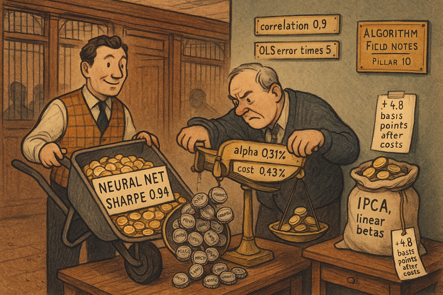
On the non-microcap book, 0.50% times the Gu-Kelly-Xiu neural net's turnover of 0.869 costs 0.4345% a month. Its Fama-French six-factor alpha on that book is 0.312%. The ticket is larger than the alpha. Instrumented principal components, the linear model that lets betas move with firm characteristics, posts a six-factor alpha of 0.613% against a cost of 0.565% and clears by 0.048 percentage points, 4.8 basis points a month. Doron Avramov's lecture is the algebra under that split. The old article "Does ML Actually Help Asset Pricing? Kelly's 20%, Not 2–3×" already showed the headline Sharpes are fragile. This is the companion ledger, plus the mean-squared-error formula that forces the shrink before anyone sorts a portfolio.
What this actually is
You run a US equity book. Someone offers a signal built from 94 firm characteristics and a neural net, and quotes a long-short Sharpe near 1. You need the Sharpe that remains once the book is cut to stocks above the 20th NYSE size percentile, and once you pay half a percent for every unit of the book you turn over in a month.
The lecture does two concrete things. It writes the mean squared error of ordinary least squares as residual variance times the trace of the inverse of X-transpose X, which blows up when characteristics move together, and that blow-up is the reason to shrink. It then files the machines traders argue about into two pricing stories: forecast each stock's beta on a few factors, or build one discount factor as a portfolio of the stocks.
Picture a surveyor with two tape measures aimed almost the same way. Each tape is fine alone. A small wobble in one reading becomes a large wobble in how much length you assign to each direction. Shrinkage is the surveyor pulling that split back toward a dull answer. Beta pricing and the discount factor are two choices of what "dull" was allowed to mean before the tapes came out.
If the ledger holds, you keep the linear instrumented-factor sleeve on names large enough to trade. If the ledger is wrong, you have skipped a nonlinear premium in liquid stocks, and 4.8 basis points a month will not pay for that miss. The old article "The SDF View: One Equation Behind Every Factor Model" is the same discount factor from the Kelly lecture. Avramov writes the cost column beside it.
The trace that blows up
Two predictors at a correlation of 0.9 make the OLS coefficient error 5.263 times the orthogonal case. That ratio is the whole case for a penalty.
Avramov starts from ordinary least squares because every later machine is a repair of it. With spherical residuals of variance sigma-squared, and a fixed predictor matrix X with T rows and M columns, the mean squared error of the coefficient vector is residual variance times a trace.
$$ \mathrm{MSE}(\hat\beta) = \sigma^2 \, \mathrm{tr}\!\left[(X'X)^{-1}\right] $$
Read it as: sigma-squared is the residual variance, in return-squared units. X-transpose X is the M by M Gram matrix of the predictors. The trace of its inverse adds one term per coefficient, and each term is large when that direction in X is thin. Mean squared error here is the expected sum of squared coefficient errors, so the unit is coefficient-squared. The old article "The Mathematics of Machine Learning, for Traders" is the general split of that error into variance plus bias squared. OLS is unbiased under the lecture's assumptions, so the trace is the whole error. Work it with two predictors and T = 240 months, columns scaled so X-transpose X equals 240 times the correlation matrix. At zero correlation the trace is 2/240 = 0.008333. At correlation 0.9 the eigenvalues of the correlation matrix are 1.9 and 0.1, and the trace is (1/1.9 + 1/0.1) / 240 = 10.5263 / 240 = 0.04386. The ratio of the two traces is 1 / (1 - 0.9 squared) = 1 / 0.19 = 5.263. Same residual variance, 5.263 times the coefficient error. At correlation 0.99 the factor is 1 / (1 - 0.99 squared) = 50.25. Firm characteristics live in that region. Size, value, profitability, and investment do not point in orthogonal directions.
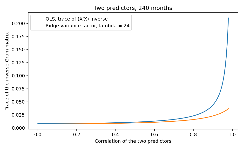
The orange line is a ridge penalty of 24, which is 10% of T, added to the diagonal before the inverse. At correlation 0.9 its trace is 0.0229, against the OLS trace of 0.04386, so the variance piece falls to about half. Read the orange line as the variance piece only. Ridge is biased, so its full mean squared error also carries a squared-bias term the trace leaves out. The chart's job is the blue line: the variance was about to explode, and a small diagonal load stops the explosion.
The same shrinkage, written as a discount factor
The question here is where the penalty sits inside a pricing equation, and which first-order condition the lecture's slope formula obeys.
Hoerl and Kennard's ridge estimator adds lambda times the identity to X-transpose X before inverting. As lambda goes to 0 you recover OLS. As lambda goes to infinity every slope goes to 0. The useful object is the weight on each principal component of the fitted values: eigenvalue j over (eigenvalue j plus lambda). In the two-predictor example the eigenvalues of X-transpose X are 24 and 456. With lambda = 24 the small component is kept at 24/48 = 0.5, and the large one at 456/480 = 0.95. Ridge barely touches the direction the data can see, and it cuts the thin direction in half.
Avramov then writes the same penalty as a prior on the stochastic discount factor. The kernel, in the Hansen-Jagannathan projection the lecture uses, is one minus a portfolio of demeaned returns.
$$ M_t = 1 - b'(r_t - \mu) = 1 - \mu' V^{-1} (r_t - \mu) $$
Read it as: M_t is the discount factor, a pure number. r_t is the vector of excess returns, mu is their mean, same units as return. b is the vector of portfolio weights. V is the covariance matrix of those returns. The second equality sets b equal to V-inverse times mu. One asset, V = 0.04 (monthly variance), mu = 0.01. Then b = 0.01 / 0.04 = 0.25. A month that realizes 0.06 has a demeaned return of 0.05, the portfolio inside M is 0.25 times 0.05 = 0.0125, and M = 1 - 0.0125 = 0.9875. The discount factor is low when the high-mean asset pays off.
Check the first-order condition against the lecture's own line. The population identity E[M r] = mu - V b. Plug in b = V-inverse mu and that product is zero: the kernel prices the excess returns. The lecture writes the condition as E[M (r - mu)] = 0. That residual equals -mu, which is -0.01 in the example, and the only b that sets it to zero is b = 0. The slope formula in the slide is the standard one. The residual printed next to it does not deliver that slope. Keep the formula, and treat the printed Euler residual as a slip in the notes.
Kozak, Nagel, and Santosh put a normal prior on b and the posterior mean is ridge.
$$ E(b) = (V + \lambda I)^{-1} \hat\mu, \qquad \lambda = \frac{s^2}{T \sigma^2} $$
Read it as: mu-hat is the sample mean return. s-squared is the trace of V, a sum of variances. T is the number of months. Sigma-squared here is the prior's confidence knob, a different object from the residual variance in the OLS section. Lambda is the ridge penalty, in variance units. With V = 0.04, mu-hat = 0.01, T = 120, and sigma-squared = 1/120, lambda = 0.04 / (120 times 1/120) = 0.04. The posterior weight is 0.01 / (0.04 + 0.04) = 0.125, half the OLS weight of 0.25. You gave up unbiasedness and cut the position in half.
The lecture's eta parameter decides whether that prior's expected squared Sharpe grows with the number of components. Eta = 2, the case that makes the prior on b independent of V, sets the expected squared Sharpe equal to sigma-squared. In the example that is 1/120 per month, and the root-mean-square Sharpe is the square root of 0.1, which is 0.316 annualized. Eta = 1 multiplies by the number of components. Feed the same sigma-squared into 94 managed portfolios, the characteristic count the lecture hands Kozak, and the expected squared Sharpe is 94 / 4.8 = 19.583 per month. The root-mean-square Sharpe is the square root of 19.583 times 12, equal to 15.33 annualized. That 15.33 is an illustration of their formula under a monthly covariance. The lecture does not print it. You would not sign the eta = 1 prior at that width. Eta = 2 is the prior that stays humble, and it is the prior that lines up with ridge.
Beta pricing versus the kernel
The question is which restriction each famous machine imposes. They run on different samples, so a ranking is the lecture's composite.
Avramov sorts them on one page. Gu, Kelly, and Xiu (2020) is a reduced form: a three-layer net, 32, 16, and 8 neurons, predicting the next return from firm characteristics and macro variables, with no pricing restriction. The predictor count is (8 + 1) times 94 characteristics, plus 74 industry dummies, which is 920. A toy net with 4 inputs, 5 hidden units, and 1 output has (4 + 1) times 5 plus 6 = 31 parameters, their own count, so you can see the scaling before the real net. Training is 1957 to 1974, validation 1975 to 1986, and the out-of-sample window is 1987 to 2017.
Kelly, Pruitt, and Su price with betas. The conditional loading is linear in characteristics, and the factors are latent.
$$ r_{i,t+1} = \beta_{i,t}' f_{t+1} + \varepsilon_{i,t+1}, \qquad \beta_{i,t}' = x_{i,t}' \Gamma_\beta $$
Read it as: r is stock i's excess return next month. f is a K-vector of latent factor returns. beta is that stock's loading, dimensionless if f is a return. x is the stock's characteristics, including a one for the intercept. Gamma-beta is an M by K matrix shared across stocks. No alpha in this line: the characteristics move the loading, and the loading times the factor is the whole expected return. Their implementation uses 6 factors and 94 characteristics, re-estimated every month, out of sample 1987 to 2017. Work one factor. A stock with x = (1, 0.5) and Gamma-beta = (0.8, -0.4) has beta = 0.8 + 0.5 times -0.4 = 0.6. A factor realization of 0.02 (2% that month) contributes 0.6 times 0.02 = 0.012, or 1.2%, to the stock. A stock with the size coordinate at 0 has beta 0.8 and a contribution of 1.6%. The characteristic changed the loading. It did not add a separate cash intercept.
Gu, Kelly, and Xiu (2021) replace the linear map x-transpose Gamma with a neural net, two hidden layers of 32 and 16 units, and 5 latent factors. Same beta-pricing story, nonlinear loading. They call it a conditional autoencoder. Out of sample runs 1987 to 2016.
Chen, Pelger, and Zhu stay on the kernel side and let an adversary pick the moments. The discount factor is one minus a portfolio whose weights are a network of characteristics and a macro state.
$$ \min_w \max_g \ \frac{1}{N} \sum_{j=1}^{N} \left\| E\!\left[\left(1 - \sum_{i=1}^{N} w(I_t, I_{t,i}) R^e_{t+1,i}\right) R^e_{t+1,j}\, g(I_t, I_{t,j})\right] \right\|^2 $$
Read it as: w is the discount-factor portfolio, a weight per stock, a function of macro information I_t and stock information I_{t,i}. g is the adversary's instrument, also a function of those inputs, scaled to sit between -1 and 1. The object inside the norm is a pricing error: discount factor times excess return times instrument, averaged over time, then squared and averaged across stocks. The modeler picks w to shrink those errors. The adversary picks g to inflate them. They alternate. Hansen and Jagannathan (1997) motivate the minimax: when the kernel is only a proxy, minimizing the largest pricing error pulls it toward an admissible kernel in least squares. A one-month sketch of the portfolio inside M, with the expectation left to the sample average: weights 0.6 and -0.4, excess returns 0.03 and -0.01, portfolio return 0.6 times 0.03 plus -0.4 times -0.01 = 0.022, so M = 0.978. Their benchmark uses on the order of 10,000 stocks and 8 instruments, about 80,000 instrumented assets, so the adversary can only "win" on mispricing that hits a large share of names. Training is 1967 to 1986, validation 1987 to 1991, out of sample 1992 to 2016, on 46 firm characteristics plus 178 macro predictors.
Those windows do not match, and the stock sets do not match either. The Gu-Kelly-Xiu, IPCA, and autoencoder samples cover 21,882 NYSE, AMEX, and Nasdaq names, 5,117 to 7,877 in a given month. Chen-Pelger-Zhu cover 7,904 names, 1,933 to 2,755 a month. Read a ranking of their full-sample spreads as that composite.
The book you can trade
The question is which of those spreads survives the names an institution can hold, after a turnover charge. The figures are Avramov, Cheng, and Metzker's, printed as the lecture's appendix. The lecture's reason for throwing out small names is the anomaly record it cites. Harvey, Liu, and Zhu count 296 published anomalies and judge 27% to 53% of them false discoveries. Hou, Xue, and Zhang find that 82% of 452 anomalies lose significance once microcaps are out and the portfolios are value-weighted.
On the full sample the lecture's own bars read 0.95% a month for IPCA (six-factor alpha 0.62%), 1.56% for the neural net (alpha 0.92%), and 2.18% for the adversarial kernel (alpha 1.87%). The alpha column matches the printed table at two decimals: 0.624, 0.916, and 1.867. Sharpes in that table are 0.967, 0.944, and 1.225, against a market Sharpe of 0.527. A market Sharpe of 0.53 is an annualized equity number, so read the Sharpe column as annualized. Read the return and alpha columns as percent per month: dividing the neural net's full-sample alpha 0.916 by its turnover 0.976 recovers the printed break-even of 0.94, and that division only lands if alpha and turnover share a month.
Drop stocks below the 20th NYSE size percentile and the table changes shape. Neural-net Sharpe goes from 0.944 to 0.644. Six-factor alpha goes from 0.916 to 0.312, a 66% cut. The adversarial kernel goes from Sharpe 1.225 to 0.839, and from alpha 1.867 to 0.548, a 71% cut. The conditional autoencoder's alpha goes from 0.746 to 0.387, and (0.746 - 0.387) / 0.746 = 48%, which is the lecture's own "48% lower" on that method. IPCA goes from Sharpe 0.967 to 0.978, and from alpha 0.624 to 0.613, a 1.8% cut. The linear beta model's alpha barely moves when the microcaps leave. The lecture also states that value-weighting the neural-net spread cuts performance 48% relative to equal-weighting. That 48% is the lecture's sentence. The figure behind it lacks labels tight enough to recompute the percent from the bar heights.
Turnover is why the alpha that remains fails to cover the ticket. One-way monthly turnover is 0.976 for the neural net, 1.664 for the adversarial kernel, 1.186 for IPCA, and 1.565 for the autoencoder, against under 0.10 for size and value in the lecture's comparison set. The non-microcap break-evens, alpha divided by turnover, print as 0.36, 0.34, 0.54, and 0.26 percent per unit of turnover. Recomputed: 0.312 / 0.869 = 0.359, 0.548 / 1.625 = 0.337, 0.613 / 1.130 = 0.542, 0.387 / 1.478 = 0.262. The lecture's rounding matches.
$$ \text{cost} = 0.50\% \times \text{turnover}, \qquad \text{net} = \text{FF6} - \text{cost} $$
Read it as: 0.50% multiplies one-way turnover, so a turnover of 1.130 produces a charge of 0.565%. Turnover is a fraction of the book traded in the month. FF6 is the six-factor alpha in percent per month. Net is alpha left after that charge, same units. Non-microcap turnover is 0.869, 1.625, 1.130, and 1.478. Costs are 0.4345, 0.8125, 0.565, and 0.739 percent per month. Nets are 0.312 - 0.4345 = -0.1225, 0.548 - 0.8125 = -0.2645, 0.613 - 0.565 = +0.048, and 0.387 - 0.739 = -0.352. One method is positive.
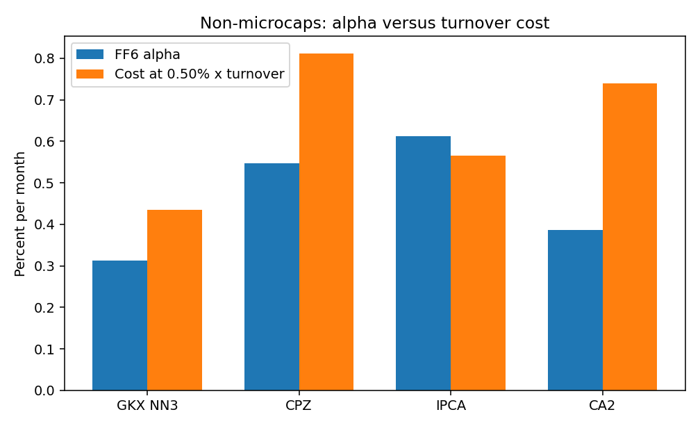
The lecture's chart of the same comparison labels the bars 0.31 against 0.43, 0.55 against 0.81, 0.61 against 0.57, and 0.39 against 0.74. Same arithmetic, one-decimal labels. IPCA is the only bar pair where alpha stands above the cost. The full-sample neural-net break-even of 0.94% looked like it could pay this rate. That 0.94 includes the microcaps. On the tradable book the break-even is 0.36%, and 0.50% is above it.
The edge also shows up in the months when arbitrage is expensive. On the neural-net long-short the lecture prints a high-sentiment coefficient of 1.534 (t = 2.43) and, in a sibling specification, a high-VIX coefficient of 1.851 (t = 2.85). IPCA and the autoencoder, the lecture says, show low time-series variation and mixed evidence in those states. The deep reduced form and the adversarial kernel earn more of their keep when the market is hard to trade. That is the same fact as the microcap result, moved from the cross-section to the calendar.
A stock pick inside the industry
The question is whether the forecast is picking stocks or picking industries. For the neural net, the lecture's split says stocks.
Define the unconditional long-short from the gap between each stock's predicted return and the predicted market, scaled so the positive weights sum to one.
$$ WML_{t+1} = \frac{1}{H_t} \sum_{i=1}^{N_t} (\hat R_{i,t} - \hat R_{m,t}) R_{i,t+1}, \qquad H_t = \frac{1}{2} \sum_{i=1}^{N_t} |\hat R_{i,t} - \hat R_{m,t}| $$
Read it as: R-hat is the model's predicted return, R is the realized return, both in the same units. The market prediction is the cross-sectional average of the predictions. H is half the sum of absolute gaps, so dividing by H turns the gaps into long-short weights. The lecture then splits each gap into a within-industry piece and an across-industry piece, and the two pieces add back to the unconditional spread. Three stocks, predictions 4%, 2%, and 0%, so the market prediction is 2% and H = 2. Realized returns 5%, 1%, and -3%. Unconditional payoff: (2/2) times 5 + (0/2) times 1 + (-2/2) times -3 = 8 percent that month. Put the first two stocks in one industry, predicted industry mean 3%, and the third alone in another. Within-industry payoff is 2 percent. Across-industry payoff is 6 percent. Sum is 8. In this toy the industry bet is most of the money. In the lecture's full sample the mix flips: the within-industry piece is 84% of the raw neural-net payoff and 93% of the risk-adjusted payoff. The signal is a stock pick inside an industry. The longs the lecture describes line up with the usual anomaly book: small, cheap, illiquid, low recent issuance. Two exceptions, high investment and high idiosyncratic volatility, are where they say the nonlinearity is doing something a linear sort would miss.
None of that makes the 4.8 basis points a strategy. It tells you which restriction was binding. A reduced-form net and an adversarial kernel find a large in-sample-looking spread, then give most of it back once microcaps, distress, and a half-percent turnover charge are in the ledger. A linear beta that is allowed to move with characteristics keeps a thin residual. The old article "Does ML Actually Help Asset Pricing? Kelly's 20%, Not 2–3×" put the practitioner's 20% next to the published 2-to-3 times. Avramov prices the turnover, and on the tradable book the linear model is the one with a positive net. If you deploy one of these four, deploy IPCA. The neural net's full-sample Sharpe is the wrong number to budget.
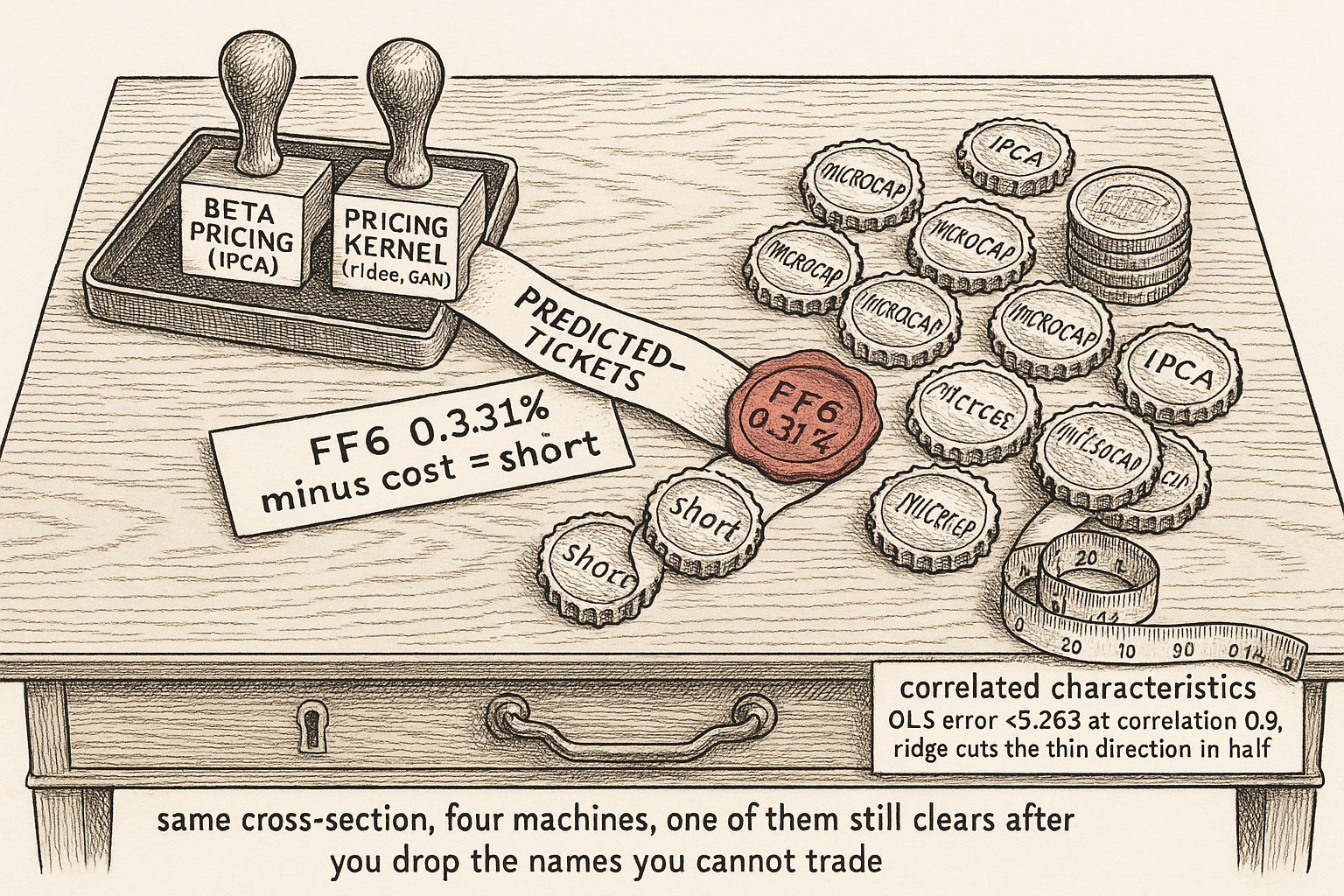
KEY POINTS
- OLS mean squared error equals sigma-squared times the trace of (X-transpose X) inverse. Two predictors, 240 months, correlation 0.9: the trace is 0.04386 against 0.008333 when the columns are orthogonal, a factor of 5.263. That explosion is why the lecture shrinks.
- Ridge is the same object as a normal prior on the discount-factor weights. M equals 1 minus b-transpose times (r minus mu), with b equal to V-inverse mu. The lecture's printed condition E[M (r minus mu)] equals 0 does not deliver that b. The condition that does is E[M r] equals 0. Treat the printed residual as a slip.
- With the prior that sets lambda to 0.04, an OLS weight of 0.25 shrinks to 0.125. The eta-equals-2 prior keeps expected squared Sharpe at sigma-squared (0.316 annualized in the worked example). Eta equals 1, on 94 portfolios with the same knob, implies a root-mean-square Sharpe of 15.33. That 15.33 is an illustration of the formula. The lecture does not print it.
- The four machines are two stories. IPCA and the conditional autoencoder are beta pricing, linear versus a net. Kozak-style ridge and the Chen-Pelger-Zhu adversary are the kernel. Gu-Kelly-Xiu is a reduced form with 920 predictors and no pricing restriction. The out-of-sample windows and the stock universes (21,882 names versus 7,904) do not match.
- On non-microcaps, a 0.50% times turnover charge leaves the neural net, the adversarial kernel, and the autoencoder with negative nets (-0.1225, -0.2645, -0.352 percent per month). IPCA's six-factor alpha of 0.613 against a cost of 0.565 is the only positive net, +0.048 percent per month. Its Sharpe does not fall when microcaps leave (0.967 to 0.978).
- The neural-net payoff is a within-industry stock pick: 84% of the raw spread and 93% of the risk-adjusted spread. High-sentiment and high-VIX months add 1.534 (t = 2.43) and 1.851 (t = 2.85) to that long-short. The alpha lives where the book is hardest to trade.