3.52 Every Edge Has a Half-Life: A Decay-Constant Taxonomy
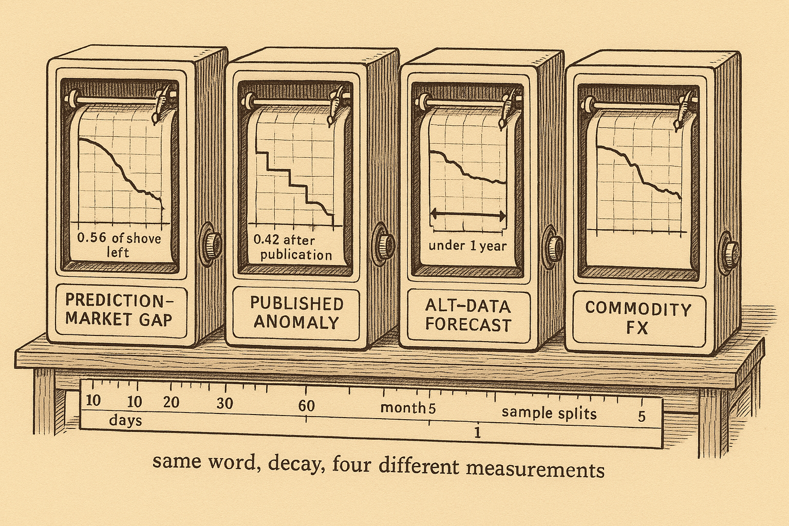
Edge half-life is a measured clock: a prediction-market gap keeps 56% at day 60, published anomalies keep 74% out of sample, and commodity-FX slopes die by month five.
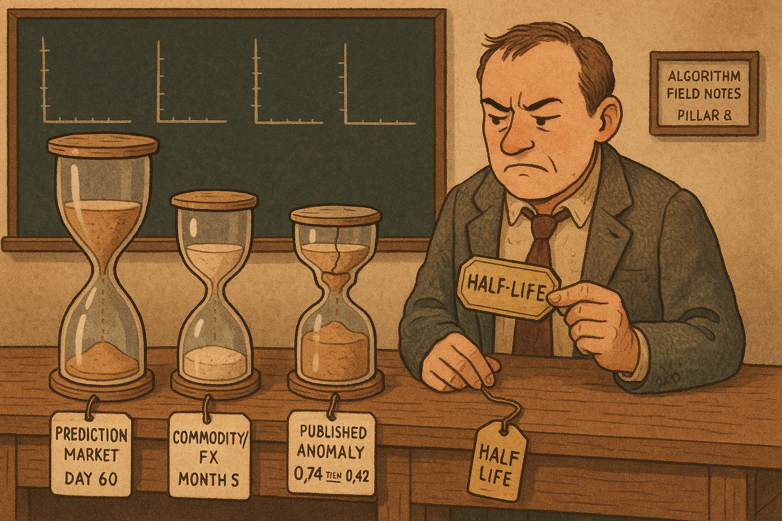
Rasooly and Rozzi pushed the price of 817 prediction markets by 5 percentage points, and the gap between the markets they pushed up and the markets they pushed down was still there 60 days later. That leftover path is an impulse response: you hit the system, then you write down what is left at each lag, and the time it takes to die is a constant you can put on a row. A published stock predictor, an alternative-data earnings forecast, and a commodity-currency underreaction each die on a different row, on a different clock. The old article "Why Systems Work Until They Don't" already says you switch a system off when its life is over. You pick the day from the row, once you have measured which clock the edge runs on.
A half-life fitted at day 60 still leaves 93% of the gap at day 7
The old article "How Manipulatable Are Prediction Markets? The Field Experiment" already walks the design. Here you only need the path. Each market was shoved up 5 percentage points, shoved down 5, or left alone, so the design gap between the yes group and the no group is 10 percentage points. They then estimate, at each lag t,
$$ p_{t,i} = \beta_0 + \beta_1 \mathbb{I}_{Y,i} + \beta_2 \mathbb{I}_{C,i} + \beta_3 p_{-1,i} + u_i $$
p is the price in market i at lag t, the yes dummy marks the markets they pushed up, the control dummy marks the markets they left alone, and p at minus 1 is the price in the hour before the bet. The no group is the omitted category, so β1 is the yes-minus-no gap after that pre-trade price is taken out. You store the fraction of the design gap that is still there:
$$ r(t) = \frac{\beta_1(t)}{0.10} $$
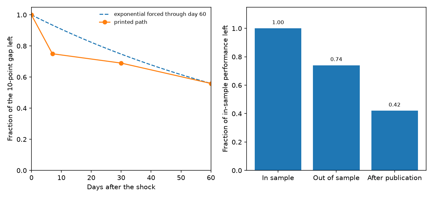
β1 is in the same units as the price, a probability, and 0.10 is the 10-point design gap, so r is a pure fraction. At one week they summarize the reversion as 25%, which leaves r(7) = 0.75, a gap of 7.5 points. At 30 days the gap has fallen to 6.9 points, so r(30) = 0.069 / 0.10 = 0.69, and the extra reversion over those three weeks is 6% of the original gap. At the day-60 snapshot the full-sample coefficient is 0.0559, so r(60) = 0.0559 / 0.10 = 0.559, which is the 44% reversion they report from a coefficient they round to 0.056. Markets still open, 771 of the 817, print 0.0586, so r = 0.586 and reversion of 41%. The first hourly print already sits a little under 10 points, because some reversion happens inside the hour of the trade. They still divide by the 10-point design gap: the 31% at day 30 is (0.10 − 0.069) / 0.10 = 0.31.
A half-life is what you get if you force that fraction through an exponential.
$$ r(t) = e^{-t/\tau}, \qquad \tau = \frac{-t}{\ln r(t)}, \qquad t_{1/2} = \tau \ln 2 $$
τ is the time constant, the lag at which an exponential has fallen to about 37% of its start, and the half-life is τ times the natural log of 2, the lag at which it has fallen by half. Plug in the day-60 fraction. ln(0.559) = −0.5816, so τ = 60 / 0.5816 = 103.2 days, and the half-life is 103.2 × 0.693 = 71.5 days. That same curve, evaluated at day 7, is e to the power of −7/103.2, which is 0.93. The market had already given back a quarter of the gap by then. The exponential that matches only the week-1 point goes the other way: ln(0.75) = −0.2877, so τ = 7 / 0.2877 = 24.33 days and the half-life is 24.33 × 0.693 = 16.9 days, and by day 60 that curve is at e to the power of −60/24.33, which is 0.085, against the measured 0.559. One constant cannot pass through both dates. Their own baseline simulation, 11 traders and a shock from 0.50 to 0.55, settles after giving back only about 40% of the shove, so a curve that has to decay all the way to zero was already the wrong shape.
The constant also depends on which market you hit. Their week-1 table, divided by the same 10-point gap they use when they call the total-volume split 31% versus 19%, puts the above-median 24-hour-volume gap at 0.049, which is 51% reversion, against 0.081 and 19% reversion below the median. The difference has a p-value of 0.041. Markets duplicated on Metaculus give back 47% in a week, against 23% for the rest, and that contrast is only significant at the 10% level. Above-median trader count gives back 33%, against 17% below, with a p-value of 0.056. They describe the active markets as running on a faster clock. Store the row conditional on that clock. The full-sample 25% mixes a group that has given back about half with a group that has given back 19%.
The further drop from 6.9 points at day 30 to 5.59 points at day 60 is 1.31 points. The day-60 level, 0.0559 divided by its standard error of 0.0135, is 4.1, so the gap is still easy to tell from zero. They do not test whether the decay sped up or slowed down over that second month. The slowdown they do claim is the earlier one: 25% of the gap in week one, and 6% over the three weeks after that.
Publication cuts the predictor in two different steps
Arakelian and coauthors, in the discussion of what a valid backtest has to survive, report a result of McLean and Pontiff: stock-portfolio predictors come in 26% lower out of sample than in sample, and 58% lower after publication. The next sentence in that paper maps the first cut onto in-sample overfitting and the second onto other people trading the published idea. The old article "Alpha Decay Is Just Competition (and Papers Lie)" is the second cut. The first cut happens before anyone else has read the paper.
$$ h = \frac{\text{performance}_{\text{later}}}{\text{performance}_{\text{in sample}}} $$
h is the fraction of the original performance number that is left after you change the sample. A 26% reduction means h = 1 − 0.26 = 0.74. A 58% reduction means h = 1 − 0.58 = 0.42. Take a predictor that earned 10% a year inside the original sample. Out of sample it earns 10 × 0.74 = 7.4% a year. After publication it earns 10 × 0.42 = 4.2% a year. Both ratios are unitless, and both are measured against the in-sample number, which is how that paragraph phrases them. h has no lag in it. The 26% is a level change between samples, and the citation does not say how many months that change took.
The same paragraph prints two more cuts and one dissent. Suhonen, Lennkh, and Perez find a median deterioration of 73% in the Sharpe ratio from backtest to live trading, across 215 smart-beta strategies sold by banks, so the median live Sharpe is 1 − 0.73 = 0.27 of the backtest Sharpe. A backtest Sharpe of 1.00 has a median live Sharpe of 0.27. Falck, Rej, and Thesmar record a 50% decline in systematic strategies after publication. Jensen, Kelly, and Pedersen, cited in the same paragraph, find a high degree of validity for factor strategies after publication, in the US and abroad. The 0.42 row is a citation inside a survey, with a conflicting citation next to it. The old article "Building a Statistically Valid Backtest: The Checklist Nobody Runs" already tells you to haircut the backtest before you believe it. The haircut is a regime ratio, with no clock attached, and the survey disagrees with itself on the post-publication step.
Alternative data loses its grip as the horizon gets longer
Chuan Shi's factor-investing deck summarizes Dessaint, Foucault, and Frésard on what happens to analyst earnings forecasts once short-horizon data gets cheap. The object they compute, for a date, an analyst, and a horizon of h months, is a cross-sectional regression of realized earnings on that analyst's forecasts, both scaled by the firm's assets:
$$ \frac{\text{Earnings}_{j,h}}{\text{Assets}_j} = \alpha + \beta \frac{\text{Forecast}_{j,h}}{\text{Assets}_j} + e_{j,h} $$
j runs over the firms that analyst covers. The R-squared of that regression is the fraction of cross-sectional variance in scaled earnings that lines up with the scaled forecasts. Average those R-squareds across dates and analysts and you have the informativeness of horizon h. Work it on three firms. Scaled earnings are 0.10, 0.06, and 0.03, so the mean is (0.10 + 0.06 + 0.03) / 3 = 0.0633. Scaled forecasts are 0.09, 0.07, and 0.02, so the mean is 0.0600. The squared deviations of the forecasts sum to 0.03² + 0.01² + (−0.04)² = 0.0026. The cross product of forecast deviations and earnings deviations is 0.00240. The slope is 0.00240 / 0.0026 = 0.92, and the R-squared of that fit is 0.90. A horizon whose R-squared sits near 0.90 is a forecast you can use. A horizon whose R-squared sits near 0.30 leaves most of the cross-section in the residual.
The deck's chart of that R-squared against horizon, for 1983 to 2017, is drawn on an axis marked from 20 to 100 in percent. The line starts near 90, an R-squared of about 0.90, and finishes near 30 at 60 months, an R-squared of about 0.30. The deck does not print those coordinates; they are read off the figure. The load-bearing printed fact is elsewhere: across 26 academic papers, alternative-data sources such as social media and satellite imagery generally have a forecast horizon of less than one year. After 2000, when that kind of data started to show up in US equities, short-horizon accuracy rose and long-horizon accuracy fell. On the two-period chart the post-2000 line starts above the 1983 to 1999 line and finishes below it, and the two meet somewhere short of three years. Again the endpoints are read off the figure, not typed in the deck. The mechanism the deck states is an effort shift. Alternative data cuts the cost of the near-term forecast, analysts spend more of a fixed budget there, and the far horizon pays for it.
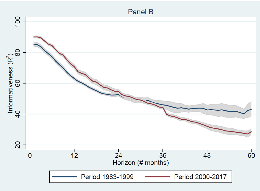
A Chinese sample in the same deck, analyst forecasts from 2012 to 2023, splits at 2016 and tells the same qualitative story: short-horizon accuracy improved in the later period, the two-year horizon got worse, and horizons past two years did not separate. No coordinate table there either. What you take to the desk is the horizon the data was built for. A satellite series whose papers stop inside a year is being asked to do a job it was not measured on, once you point it at a three-year earnings number. The R-squared is forecast accuracy. A fall from about 0.90 to about 0.30 is a loss of informational grip, and the object on the page is still an R-squared.
The commodity slope is gone after five months
Jeanneret runs a monthly panel on eight currencies whose exchange rates move with their own commodity export prices, from January 1985 to April 2020. The exchange rate is dollars per unit of foreign currency, so a rise is an appreciation of the commodity currency. For a horizon of k months,
$$ \frac{1}{k}\Delta s_{i,t+k} = \alpha_{i,k} + \delta_k \Delta \mathrm{CEP}_{i,t} + \theta_k x_t + u_{i,t+k} $$
Δs is the log change in the exchange rate from month t to month t+k, CEP is the standardized log change in country i's export-weighted commodity price index, x is a set of controls dated t, and α is a currency fixed effect, a separate intercept per currency. Dividing by k puts the average monthly move on the left side. The cumulative move is a separate product, k times the slope. With the full control set, the one-month slope is δ1 = 0.39 with a t-statistic of 3.48, so the standard error is 0.39 / 3.48 = 0.11. A one-standard-deviation rise in export prices lines up with a 0.39% appreciation over the next month. Twelve times 0.39 is 4.68. The paper prints that product as 4.7% in the body and as 4.70% in the introduction. The introduction's 4.70 sits 0.02 above 12 × 0.39. Keep 0.39, and treat 4.70 as a rounding print.
The controls are the one-month interest differential, the real exchange rate, last month's exchange-rate change, the dollar factor, aggregate FX volatility, the TED spread (LIBOR minus the three-month Treasury yield), the VIX, and an NBER recession dummy. Standard errors are Driscoll-Kraay, built to stay valid when currencies move together and when months are serially correlated. The sample shortens to January 1986 once the TED spread or the VIX is included. CEP is the predictor that stays significant. The others, apart from the real exchange rate, do not.
Because the left side is already divided by k, the cumulative appreciation implied by a slope is the slope times the horizon.
$$ C(k) = k \, \delta_k $$
C is in percent per standard deviation of the commodity move, since δ is. At one month, C(1) = 0.39%. Suppose the entire adjustment landed in that first month and nothing followed. Then the five-month regression, which divides the same 0.39% cumulative move by 5, would print δ5 = 0.39 / 5 = 0.078. A falling slope is partly that arithmetic. It is also, on their figure, a loss of statistical grip.
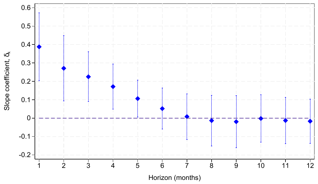
The slope is positive and significant at the short end and, in their words, negligible after five months. The month-5 interval on the figure covers zero, so 0.078 is not separated from no effect on the plot they drew. Because C(k) is k times δk, a slope that cannot be told from zero carries a cumulative move that cannot be told from zero either. Risk-premium predictability, the alternative they argue against, usually gets stronger as the horizon lengthens. This one dies.
It dies where the currency is thin. Australia and Canada, with daily FX turnover above 200 billion dollars, show no predictability. The Brazilian real and the Russian ruble, around 38 billion and 48 billion dollars a day, do, along with the New Zealand dollar and the Norwegian krone. Those names trade four to eight times less than the Australian dollar. That multiple is theirs; the 200 billion dollar floor is too round to recompute it, because they do not print Australia's exact turnover. The five-month fade is the pooled panel of eight. Inside that panel the liquid names had already finished adjusting inside the month, so their one-month slope is a zero. The row you can trade is the thin-currency row, and the paper does not subtract the spread.
The day-60 marker is still at 0.56
Look at the day-60 marker. It is still at 0.56. The middle bar is 0.74 of the in-sample return, and the right-hand bar is 0.42.
The commodity slope is 0.39 at one month and its interval covers zero after five months, the deck's survey of 26 alternative-data papers puts their horizon under a year, and the median live Sharpe across 215 smart-beta strategies is 0.27 of the backtest.
Write the row before you choose the hold
Before you size, write one row. Name the shock, the object you measure, the unit of time, the fraction left at the horizon you intend to hold, and the cost of staying that long. If two dates imply two half-lives, as 16.9 days and 71.5 days do here, you store the path and you drop the single constant. If the fraction is a sample-split ratio, you store it as a ratio and you refuse to invent a calendar for it. The old article "Why the Market Does Not Repeat, But Still Rhymes" is this table. What rhymes is the shape of the response.
Then you put the cost on the same clock, which none of these papers do for you.
On the prediction-market path, the day-60 gap lives in the markets that have not resolved. The 46 markets already resolved print a yes coefficient of 0.0855 with a standard error of 0.183. Settlement to 0 or 1 wipes the manipulation gap for a reason that has nothing to do with traders leaning against it. The dollar follow-up, Sweepcash, redeemable at about one for one with a 5% fee on withdrawals, used 4-point shocks so the opening gap was 8 points, recorded about a week on 110 markets, and did not take a day-60 snapshot. On markets with positive 24-hour volume they report 43% reversion there against 51% on the play-money markets, and they say the errors are too wide to call that a faster clock. The 60-day constant is a play-money measurement. The dollar follow-up stops at about a week. Their own model says a shock of a given size should stick longer where undoing it is expensive, and they did not run that test on the large dollar markets.
On the commodity row, 0.39% in a month has to clear the spread and the position-building lag in the real, the ruble, the krone, and the New Zealand dollar. The paper's own evidence is that leveraged funds adjust slowly in those names because the market cannot absorb the size, which is why the slope exists, and also why a backtest that assumes you got filled at the mid is telling you a story about someone else's fill. Hold past five months and you are holding a slope whose interval includes zero.
On the analyst row, do not convert an R-squared path into a position. If the papers behind the series stop inside a year, your holding period stops inside a year, or you are using a different signal.
I am against pasting one decay rate onto all four rows and calling the paste a risk limit. You size the hold to the row you wrote. A hold that sits past the lag where the fraction is gone is a backtest of a signal you have already measured as finished.
KEY POINTS
- Store the manipulation gap as a path. 0.56 of the 10-point design gap is still there at day 60, so keep the path and drop the single half-life.
- Split that path by activity before you average it. Above-median 24-hour volume has reverted 51% after a week.
- Haircut a published stock predictor by the sample you are in. Multiply the in-sample number by 0.74 out of sample, and keep the post-publication step on its own row.
- Keep alternative data inside the horizon it was measured on. Across 26 papers that horizon is under a year.
- Trade the commodity-currency slope as a one-month object: a one-standard-deviation export-price move lines up with a 0.39% appreciation in the pooled panel.
References
- Why Systems Work Until They Don't
- How Manipulatable Are Prediction Markets? The Field Experiment
- Alpha Decay Is Just Competition (and Papers Lie)
- Building a Statistically Valid Backtest: The Checklist Nobody Runs
- Why the Market Does Not Repeat, But Still Rhymes
- How manipulable are prediction markets?
- Alternative Data
- A discussion paper for possible approaches to building a statistically valid backtesting framework
- Looking Under the Hood of Commodity Currency Predictability
A note on AI. The ideas, research, analysis, and conclusions in this article are my own. I use AI tools to help with editing and wordsmithing, because English is not my first language, and I am not shy about that. AI-generated ideas and AI-assisted writing are not the same thing: the first is empty slop from a generic prompt, the second is a tool for communicating years of real research more clearly. Judge the work by its substance, not by whether software helped polish the prose.