4. Market Structure Notes June 22, 2026 7 min

4.37 Calculating a Seasonal: Raw Change vs Detrended vs Standardized

Three ways to compute a seasonal, raw, detrended, and standardized, give three different curves from the same data. The method decides what the number means, and one of them quietly leaks the future.

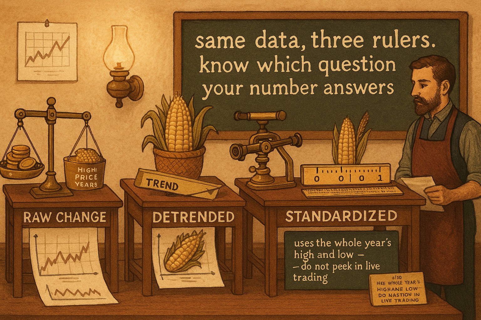
You decided corn has a seasonal. Now you have to turn that hunch into a number, and the number you get depends entirely on how you compute it. Three traders can look at the same twenty years of corn and produce three different seasonal curves, all "correct," all useless to each other, because one averaged raw price changes, one detrended first, and one standardized to a yearly range. The method is not a footnote. It decides what the seasonal even means and whether you can compare it across years or across markets.

The problem underneath is the one the article "How to Build Stationary Indicators from Non-Stationary Prices" hammered on. Price is non-stationary. Corn at \$3 a bushel in one decade and \$7 in another is the same percentage wiggle in dollars that are twice as big. Average raw dollar moves across twenty years and the high-price years drown out the low-price years, so your seasonal is really a chart of which years happened to be expensive. Every method below is an attempt to get a seasonal that says "what the calendar does" instead of "which years had big absolute prices."

Three methods, increasing in how much they correct for. Pick based on what you need the seasonal for.

Method one: raw price change

The simplest seasonal averages the price change at each calendar slot across all years in your sample. Slot can be a day-of-year, a week, or a month. For each slot you collect the change observed in every year and take the mean.

$$ \text{Seasonal}_{\text{raw}}(d) \;=\; \frac{1}{Y}\sum_{y=1}^{Y} \big( P_{y,d} - P_{y,d-1} \big) $$

Read it plainly: for calendar slot d (say, the 5th trading day of July), look at every year y, take that day's price change in dollars, and average over all Y years. Do it for every slot and you have a raw seasonal curve. It is fast, it needs nothing but prices, and for a single market over a short, price-stable window it is fine.

The flaw shows up the moment your sample spans a big change in price level. A \$0.10 move in \$7 corn and a \$0.10 move in \$3 corn count the same in dollars but are not the same event. Worse, if corn spent the back half of your sample at double the price, the recent years contribute bigger dollar swings and dominate the average. Your "seasonal" is partly a seasonal and partly a record of the price trend over the sample. That contamination is exactly why the next method exists.

Method two: detrended seasonal

Detrending removes the slow drift in price level so what is left is the wiggle around the trend. Subtract a long-term average from each price before you measure the seasonal. The long-term average is the trend; the price minus the trend is the deseasonalized-of-trend residual, and averaging that residual by calendar slot gives you a seasonal that is not riding the bull or bear market underneath.

$$ \tilde{P}_{y,d} \;=\; P_{y,d} - \overline{P}_{y}\,,\qquad \overline{P}_{y} \;=\; \frac{1}{N}\sum_{i=1}^{N} P_{y,i} $$ $$ \text{Seasonal}_{\text{detrended}}(d) \;=\; \frac{1}{Y}\sum_{y=1}^{Y} \tilde{P}_{y,d} $$

The first line subtracts a long-term average from each price. Here the average runs over the year (or a rolling long window), so each year's prices are expressed as a deviation from that year's own level. A price above its yearly average is positive, below is negative. The second line averages those deviations by calendar slot. The result tells you where in the year price tends to sit above or below its own trend, which is the actual seasonal shape with the trend stripped out.

This is the same move ATR normalization makes for volatility, described in "Why ATR Normalization Is More Than a Volatility Trick": divide out the part that contaminates the comparison so the remainder is comparable across regimes. Detrending kills the level contamination. It does not yet kill the scale contamination. A detrended seasonal in dollars is still in dollars, so a volatile high-priced year still contributes bigger deviations than a calm cheap year. If you want to average across markets, or across decades with very different volatility, you need one more step.

Method three: standardized seasonal

Standardizing rescales each year onto a common ruler so every year contributes equally regardless of its price level or its range. The straightforward version uses the year's own high and low to map price into a 0-to-1 band.

$$ S_{y,d} \;=\; \frac{P_{y,d} - \text{Low}_{y}}{\text{High}_{y} - \text{Low}_{y}} $$ $$ \text{Seasonal}_{\text{std}}(d) \;=\; \frac{1}{Y}\sum_{y=1}^{Y} S_{y,d} $$

For each year, find that year's highest and lowest price. The first line scales every price in the year to where it sits between them: 0 at the year's low, 1 at the year's high, 0.5 halfway up the range. Now a year that traded \$2 to \$3 and a year that traded \$6 to \$9 are on the same 0-to-1 scale, and neither dominates. The second line averages the scaled values by calendar slot. The seasonal now reads as "on this date, price tends to sit at, say, 0.7 of the year's range," which is comparable across years and across markets.

Standardizing buys you cross-comparability at a cost you should name out loud. Using the full-year high and low means you are peeking at the whole year to scale each day, which is look-ahead if you ever try to compute it in real time on the current, unfinished year. For research on completed historical years it is fine; for a live signal you have to scale with data available up to that bar, not the year's eventual high and low. This is the kind of subtle in-sample leakage the article "How to Build Stationary Indicators from Non-Stationary Prices" flagged, and it is easy to commit by accident when you copy a textbook seasonal formula that quietly assumes you already know the year's range.

Which one to use

Match the method to the job, and do not pretend the choice is free.

$$ \begin{array}{ll} \text{single market, short stable window} & \rightarrow \;\text{raw change}\\[4pt] \text{single market, long sample with trend} & \rightarrow \;\text{detrended}\\[4pt] \text{cross-year or cross-market comparison} & \rightarrow \;\text{standardized} \end{array} $$

Raw change for a quick look at one market where price did not move much over the sample. Detrended once your sample is long enough that the bull or bear trend underneath would otherwise leak into the seasonal. Standardized when you need years or markets on a common ruler, accepting the look-ahead caveat for live use. The three are not competing answers to one question; they answer three different questions, and the mistake is computing one while believing you measured another.

Whatever you pick, the calendar slot also matters, and it ties back to the engine. The article "The Three Engines of Seasonality: Fixed-Date, Floating-Date, and Behavioral" made the point that a floating-date seasonal has to be aligned to its event before averaging. None of these formulas fix that for you. If you average an unemployment-release effect by raw calendar date, the cleanest detrending and standardizing in the world still gives you noise, because you binned the data on the wrong axis. Get the alignment right first, then choose your computation.

A computed seasonal is an average, and an average hides its own reliability. A curve that says "up 0.7 of the range on this date" could be ten years agreeing or two huge years dragging eight flat ones. The number on the chart does not tell you which. That is the next problem, and the article "Is Your Seasonal Real or Curve-Fit? A Reliability Checklist" is where the seasonal stops being a pretty curve and has to prove it is real.

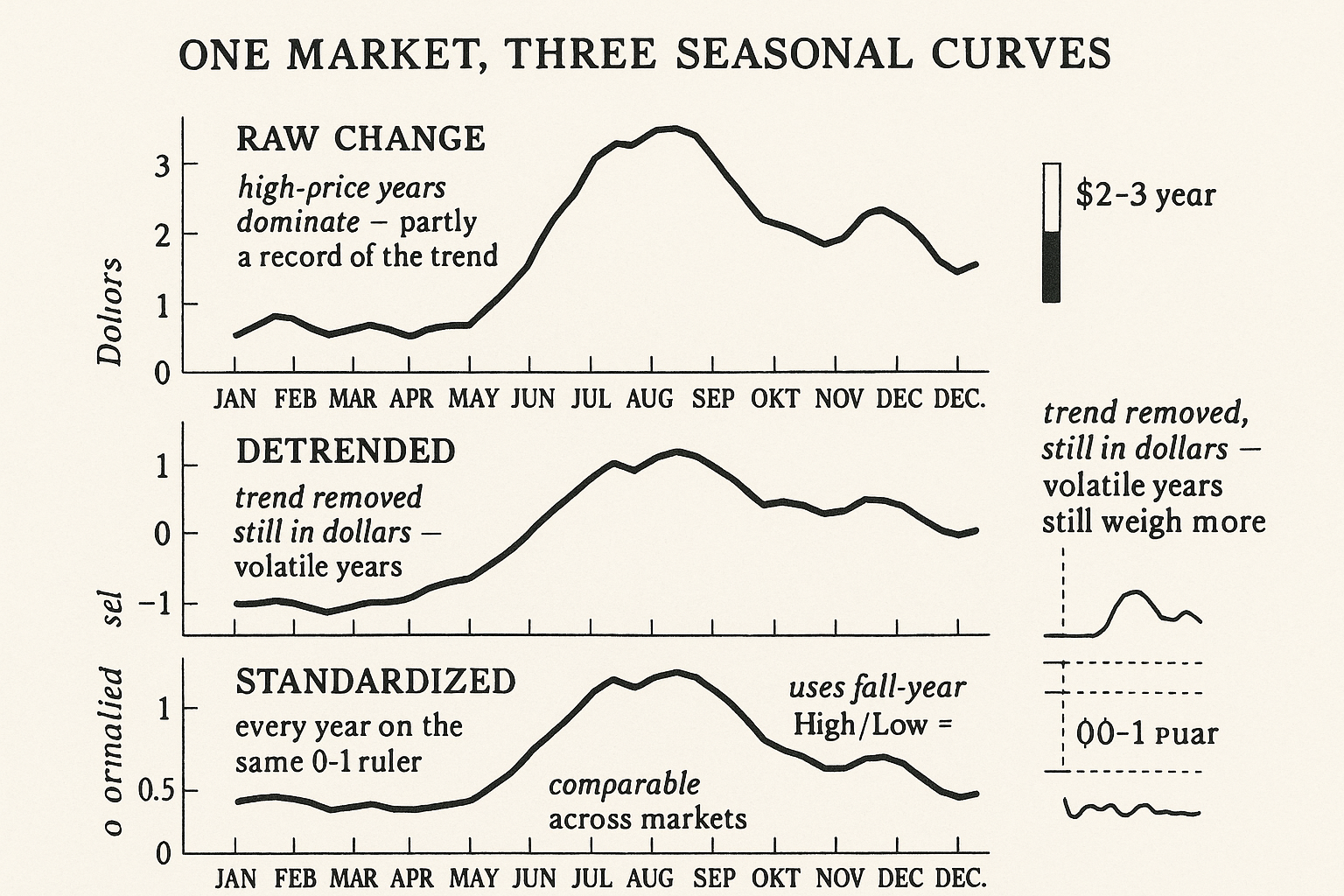
Visualizing the three computations

KEY POINTS

The method you use to compute a seasonal decides what it means. Raw change, detrended, and standardized answer three different questions; computing one while believing you measured another is the core mistake.
Raw price change averages the dollar change at each calendar slot across years. Fine for a single market over a short, price-stable window. Contaminated once the sample spans a big change in price level, because high-price years dominate the average.
Detrended subtracts a long-term average from each price before averaging by slot, so the seasonal does not ride the bull or bear trend underneath. Removes level contamination, not scale contamination.
Standardized rescales each year to a 0-to-1 band using that year's high and low, putting every year and market on a common ruler. Buys cross-comparability at the cost of look-ahead: using the full-year high/low peeks at the future if you compute it live.
Match method to job: raw for a quick single-market look, detrended for long samples with a trend, standardized for cross-year or cross-market comparison.
The formulas do not fix alignment. A floating-date seasonal must be aligned to its event before averaging, or the cleanest detrending still produces noise.
A computed seasonal is an average that hides its own reliability. Ten years agreeing and two outlier years dragging the rest produce the same curve; the curve alone cannot tell you which.