7.8 You're Modeling the Wrong Y: Label Design Beats Model Choice, Four Times
Cross-sectional stock returns: rank the monthly target and Spearman correlation goes from 0.040 to 0.107. The feature transform moves it from 0.085 to 0.092.

You fit a model to predict a return, and the research budget goes into which model. Cakici and Zaremba held the learner fixed, an equal-weighted blend of eight standard models on 147 characteristics, and changed only the target that a value-weighted decile book is sorted on. The average Spearman rank correlation of the forecast with next month's return rises from 0.040 on the raw excess return to 0.107 once that return is replaced by its cross-sectional rank. Wang's Bitcoin book, Burdorf's momentum portfolios, and Tepelyan's one-minute bars split the same way on different clocks. Write the label before you pick the architecture. The old article "Getting the Target Right: The Transform That Beats 147 Features" is the equity case of that rule.
Demean the month, then rank it
A raw excess return trains the model on the market. The panel is 35 equity markets, January 1994 to December 2024, with the forecast scored from January 2003. Each month the cross-section is the stocks on hand, about 26,215 names in a typical month, and every transform below is computed inside that month. In a down month almost every name is red, so a characteristic that lines up with "this was a bad month" gets credit for a forecast of the index.
Subtract the cross-sectional mean first. Cakici and Zaremba write the demeaned target as their equation (5).
$$ r_{i,t}^{DM} = r_{i,t} - \bar{r}_t $$
Stock i's excess return this month, minus the average excess return of every stock this month. The remainder is the relative return a long-short book holds. Work a month with a cross-section that averaged +4%. A stock that returned +6% has a raw target of +6% and a demeaned target of +2%. The same stock in a month that averaged -3%, with its own return at -1%, still has a demeaned target of +2%. The raw column called it a loser. The demeaned column calls it a relative winner, which is the only fact the decile sort uses.
Demeaning fixes the level and leaves the scale alone. A month whose returns are packed into a tight band and a month whose returns run out to the tails both enter the loss, and the wide month dominates it. Divide by that month's cross-sectional standard deviation. Their equation (6).
$$ r_{i,t}^{Z} = \frac{r_{i,t} - \bar{r}_t}{\sigma_t(r)} $$
The demeaned return, scaled so a typical name sits near one cross-sectional standard deviation. Take the +2% gap from the month above. If that month's cross-sectional standard deviation is 8%, the standardized target is 0.25. If the same +2% gap arrives in a month whose standard deviation is 2%, the target is 1.0. The quiet month is no longer a rounding error in the loss, and the wild month is no longer the whole fit.
Rank throws the gap away and keeps the order. Percentile rank is the stock's rank divided by the count of names plus one, their equation (7). The centered rank and the Gaussianized rank are that percentile mapped two ways, equations (8) and (9).
$$ r_{i,t}^{Pct} = \frac{\operatorname{rank}(r_{i,t})}{N_t + 1}, \qquad r_{i,t}^{Rank} = 2\, r_{i,t}^{Pct} - 1, \qquad r_{i,t}^{Norm} = \Phi^{-1}\!\left(r_{i,t}^{Pct}\right) $$
Rank runs from 1 to N_t inside the month, with N_t the highest return, and the +1 in the denominator keeps the percentile off 0 and off 1 so the inverse normal stays finite. Phi-inverse is the standard-normal quantile function. Work N_t = 100. The best stock has percentile 100/101 = 0.9901, centered rank 0.9802, and a Gaussianized target of 2.33. The worst stock, rank 1, has centered rank -0.9802. A name 2% above the mean and a name 20% above the mean that land in the same rank slot receive the same target. That is the magnitude the rank label discards, and it is the reason a micro-cap book later prefers the standardized column.
The same five maps applied to the 147 characteristics, standardization, an asinh compression then standardization, winsorized standardization, rank, and Gaussianized rank, are the feature side of their grid. Once the target is a rank, moving the feature map is a small residual. The old article walks that grid cell by cell.
The book label is a sign at a horizon
The label is the sign of the future mid. Wang's tape is Bybit BTC/USDT on 2025-01-30, a snapshot every 100 milliseconds, top of book out to 200 levels. He describes the label in prose and does not print a numbered expression. Binary up is a positive change in the mid over the horizon h, and the ternary label puts a flat band around zero.
$$ y^{\text{bin}}_{t} = \mathbf{1}\{m_{t+h} > m_t\}, \qquad y^{\text{ter}}_{t} = \begin{cases} \text{up} & (m_{t+h}-m_t)/m_t > \varepsilon \\ \text{down} & (m_{t+h}-m_t)/m_t < -\varepsilon \\ \text{flat} & \text{otherwise} \end{cases} $$
The mid m is the average of the best bid and the best ask. The horizon h in his tables is 100 milliseconds, 500 milliseconds, or 1 second. The indicator is 1 when the later mid is higher. The band ε is tuned so the three classes have roughly equal counts, and the source does not print the cutoff he kept. Work a mid of 103,700 that is 103,720 one second later. The change is +20, the binary label is up, and the return is 20/103700 = 1.93 basis points. A one-tick flicker that dies inside the second is the case the flat band is there to keep out of the up class. Changing the horizon, or changing the binary bit for the three-way label, rewrites the column the network is trained on.
The smooth he runs before that label looks forward. A Savitzky-Golay filter of window 21 and cubic degree fits a local polynomial and keeps the fitted level. His equation (5), with the window written as j from -10 to +10.
$$ \hat{v}_t = \sum_{j=-10}^{10} c_j \, v_{t+j}, \qquad \min_{a} \sum_{j=-10}^{10} \left[ v_{t+j} - (a_0 + a_1 j + a_2 j^2 + a_3 j^3) \right]^2 $$
Each coefficient c_j is the weight on the snapshot j steps away, solved once from the normal equations of that cubic and then reused. At a 100-millisecond clock, j = +10 is 1.0 second after the timestamp on the feature. The five nearest future weights, j = +1 through +5, sum to 0.4479. The five further future weights sum to -0.0016, so they nearly cancel, and the leak that matters is the next half-second. Raise only those five future mids by 1 dollar and the smoothed value dated now rises by 0.4479 dollars, the same sum. The single next snapshot, j = +1, carries weight 0.1059, against 0.1076 on the current print. For a 1-second label, half of the thing you claim to forecast is already inside the feature. The old article "Better Inputs Beat Deeper Nets: Crypto LOB Direction" scores the models on this tape. The label and this window are why the scores move.
Momentum's label is the next rank
Burdorf builds the same cross-sectional book four ways and changes the score. At each rebalance he longs the three highest scores and shorts the three lowest, inverse-volatility sized to a 15% annual target, across equity indices, bond indices, commodity futures, and currencies, 2000 to 2023. The old article "Momentum Is a Ranking Problem: Learning-to-Rank vs Regress-then-Rank" builds that book. The split that matters here is the column each learner is trained against. Both the network and LambdaMART see the same 22 return features, and they train on different targets.
The network is regress-then-rank. It predicts a volatility-scaled next return and is trained on mean squared error. His loss, with Y the model's score and r/σ the next return divided by a 63-day exponentially weighted volatility.
$$ L(\theta) = \frac{1}{M} \sum_{\Omega} \left( Y_t^{(i)} - \frac{r_{t,t+1}^{(i)}}{\sigma_t^{(i)}} \right)^2 $$
M is the number of asset-days in the training block. The model is punished for missing the size of the next vol-scaled return, and the ranking is something you do to the scores afterward. Work two names. The model scores them 0.20 and -0.10, and the realized vol-scaled returns are 0.50 and 0.00. The two squared errors are 0.09 and 0.01, and the loss on that pair is 0.05. A model that had the order right and the magnitudes wrong pays the same penalty as one that had the magnitudes right and the order wrong, and the book only uses the order.
LambdaMART's ground truth is the sorted rank of the next period, and the loss is a ranking loss on that rank. He writes the training objective as a sum of that loss and does not print the lambda gradient.
$$ L(\theta) = \sum_{t \in \mathcal{T}} \ell\!\left(y_t^{(i)},\, f(\mathbf{x}_t^{(i)}; \theta)\right)_{i \in \mathcal{U}} $$
y is the next-period rank inside the asset-class universe, f is the score, and ℓ is the ranking loss. The metric he optimizes, and the one he reports, is NDCG at 3, averaged over the top three and the bottom three. The gain inside that metric is 2 raised to the relevance, minus 1. He prints the average and the gain. The full discounted sum is not in the paper.
$$ \text{gain} = 2^{\text{rel}} - 1, \qquad \text{NDCG@3} = \frac{\text{NDCG@3}_{\text{top}} + \text{NDCG@3}_{\text{bottom}}}{2} $$
A relevance of 3 has gain 7. A relevance of 1 has gain 1. The top slot is worth seven times a relevance-1 name, so the metric spends its weight on where the best asset sits. He also records the practical cap: relevance above 31 overflows a 32-bit integer in the XGBoost build he used, so the universe he ranks stays at or under 31 names. Training on that rank is a different target from training on r/σ, and that target is the difference between the tree and the network.
The minute-bar label is a standardized log-VWAP
He fixes one target, and the choice of MLP, recurrent net, or Transformer is then a small move. Tepelyan's tape is Russell 3000 names in 2021, one-minute bars, a lookback of 20 bars, fit through 9 August, validated through 7 November, tested through 31 December. The target is the log change in the bar's volume-weighted average price, standardized with the training-set mean and variance. He describes it in the feature table and in the baseline section, and he does not print the expression.
$$ y_t = \frac{\log(V_t / V_{t-1}) - \mu_{\text{train}}}{\sigma_{\text{train}}} $$
V is the bar VWAP. The log ratio is the next bar over the current bar, and the training mean and standard deviation put that ratio onto a column whose training mean is 0 and whose training standard deviation is 1. Work a bar that goes from 100.00 to 100.10. The log return is log(1.001) = 0.0009995. If the training mean is 0 and the training standard deviation of that log return is 0.002, the label the network sees is 0.50. After he standardizes, the training column has mean 0.00 and standard deviation 1.00, and its excess kurtosis is 405. A Gaussian loss underweights that tail.
Every architecture emits the mean, the variance, and the degrees of freedom of a Student-t at that label, and is trained by maximum likelihood. The source does not print the density. Replacing the t with a Gaussian that keeps the same predicted mean and variance is the ablation. It changes the loss and keeps the network. He picked the VWAP log return over a close-to-close return for a concrete reason: a one-cent tick on a last trade is either exactly zero or a fake jump, and a VWAP averages the trades in the minute. A trader who knows the next bar's VWAP will be higher still has to have traded near the current VWAP to collect it. The old article "Do Intra-Bar Timestamps Carry Alpha? OHLC + Timing Features" measures what the intra-bar clock adds on top of this label.
The percentile target posts the 1.89% alpha
Look at the percentile bar on the left, and at the rightmost bar on the right.
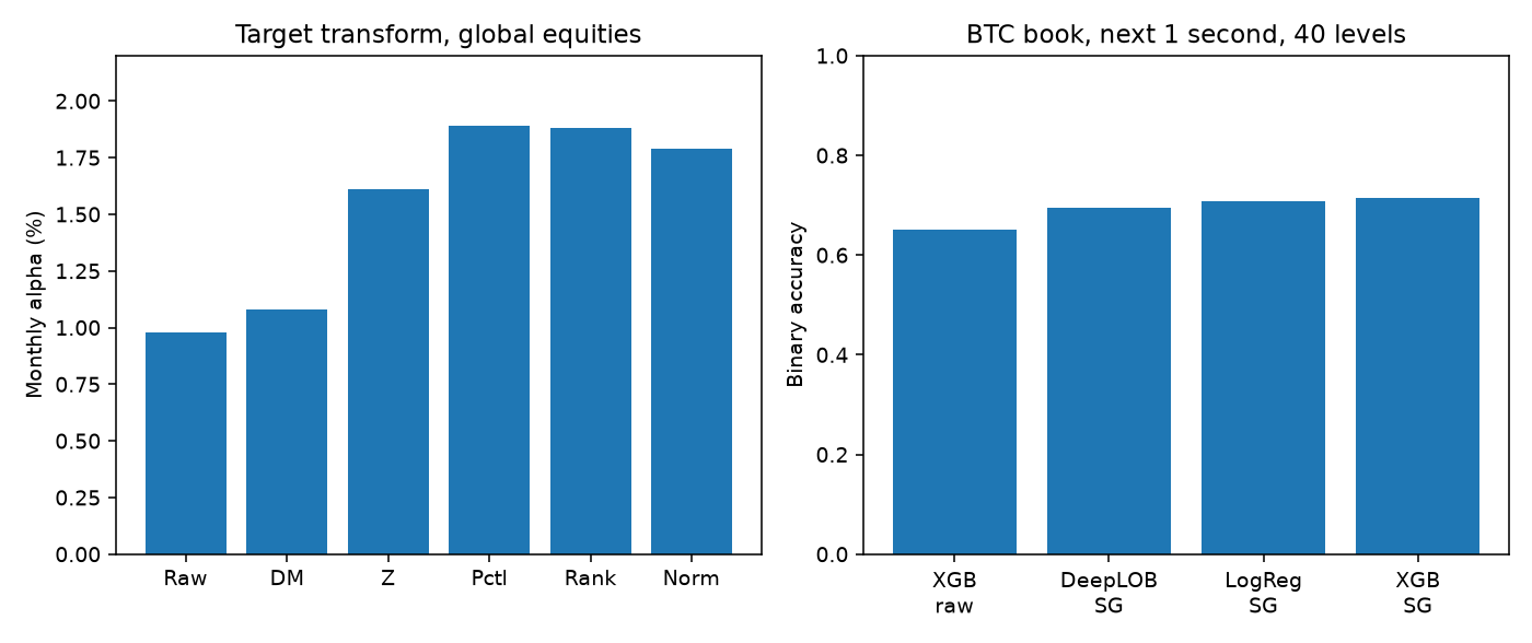
On the left, the value-weighted top-minus-bottom alpha, averaged across the five feature transforms, is 0.98% a month on raw returns, 1.61% on the standardized target, and 1.89% on the percentile target. The rest of that grid is the same shape: rank and Gaussianized targets print 1.88% and 1.79%, feature-side alphas run from 1.28% to 1.67%, average Spearman correlation moves only from 0.085 to 0.092 across those feature transforms, and average monthly returns run from 0.92% on raw to 1.62% on the rank target. The abstract's "doubles portfolio returns" matches the alpha column, 0.98 to 1.89 is 1.93 times, better than the mean-return column, which section 3.2 of the paper calls a 70 to 80 percent lift. The Spearman move in the opening, 0.040 to 0.107, is 2.68 times, which the abstract calls nearly triple. On the right, binary accuracy for the next 1 second of a 40-level book is 0.65 for XGBoost on the raw snapshots, 0.69 for DeepLOB after the Savitzky-Golay smooth, and 0.72 for XGBoost after the same smooth. Logistic regression on that smooth prints 0.71. Dropping the book from 40 levels to 5 drops that XGBoost score from 0.72 to 0.58, and the best ternary score on the same 1-second, 40-level, smoothed cell is 0.54.
The momentum comparison splits by asset class. Daily equity Sharpe is 3.40 for LambdaMART and 3.08 for the return-trained network, against -1.88 for a twelve-month sort. The printed equity cells fail to divide: mean return 0.53 over volatility 0.16 is 3.31, while the Sharpe cell is 3.40, which is what you get if volatility was about 0.156 and got rounded to 0.16. The Sharpe cell stays 3.40. Bonds give the network 1.98 and LambdaMART 1.12; currencies are 0.47 against 0.00; commodities are 0.44 against 0.08. Equity NDCG at 3 is 0.556 and 0.555, so the Sharpe gap sits outside the metric he optimized.
On the minute bars, validation negative log-likelihood on the full feature set is 0.2442 for the Transformer and 0.2480 for the MLP. Stripping the degrees of freedom, same mean and same variance, raises that Transformer's validation loss by 0.0278. Rounding those three figures to two decimals makes them identical, so they stay at the paper's precision. Test-set directional accuracy on the full feature set is 72.29%.
Run the label on a clock you can trade
Write the target inside the month, from the names you will hold, and freeze it before you retune a penalty. On a value-weighted book of large developed names the rank target is the one that led. On micro-caps the order reverses: the standardized target averages 3.23% a month and the rank target averages 2.99%, because the tails there are the signal the rank map flattens. Budget for the turnover. The rank target replaces 56.2% of the long-short book each month, against 48.9% for the raw target, and the monthly volatility of that book goes from 3.64% to 5.13%. None of those alphas is charged a spread.
On the Bitcoin book, do not center a 21-point cubic on the snapshot you are about to score. The five future weights that sum to 0.4479 sit inside a 500-millisecond forecast and inside the first half of a 1-second forecast. A causal smooth, or a smooth you can form only after those snapshots have printed, is the version you can trade. The file is one day. Taking 0.72 as a hit rate means taking a feature that can see its own label, on the snapshots that still had 40 levels.
On the momentum book, train on the rank when the book is the top three against the bottom three, and leave the 3.40 on the page. Weekly, the same equity test prints 0.54 for LambdaMART and 0.64 for the return-trained network. Weekly bonds print 0.80 for the twelve-month sort and -0.27 for LambdaMART. He reports no transaction costs, and he flags that the equity-index list may keep the names that survived. The daily Sharpe is a method comparison on a frictionless, possibly cleaned universe.
On the minute bars, use the standardized log-VWAP when VWAP is the benchmark you execute against, and size off the predicted scale rather than off the 72.29% sign rate. You cannot sell the next bar's VWAP. A close-to-close label would be a different product, and he did not run it. I am against shipping any of the four headlines as a live book until the label in the notebook is the label you can fill, and the cost sits in the same column as the alpha.
KEY POINTS
- Rank-map the monthly equity target before you swap models. Spearman correlation goes from 0.040 to 0.107, and the feature transform moves the average only from 0.085 to 0.092.
- Score the horizon and the smooth before you add a layer. On the 1-second, 40-level Bybit cell, smoothed XGBoost prints 0.72 and smoothed DeepLOB prints 0.69.
- Train the momentum book on the next rank when you only trade the top three against the bottom three. Daily equity Sharpe is 3.40 against 3.08, and the weekly prints are 0.54 and 0.64.
- Standardize the log of next-bar VWAP and keep the heavy tail in the loss. The Transformer and the MLP differ by 0.0038 in validation NLL; dropping the degrees of freedom costs 0.0278.
- Price the label's cost in the same column as the alpha. The rank target turns over 56.2% a month and runs at 5.13% monthly volatility, and the centered book smooth looks half a second ahead.
References
- Getting the Target Right: The Transform That Beats 147 Features
- Better Inputs Beat Deeper Nets: Crypto LOB Direction
- Momentum Is a Ranking Problem: Learning-to-Rank vs Regress-then-Rank
- Do Intra-Bar Timestamps Carry Alpha? OHLC + Timing Features
- Getting the Target Right in Return Prediction, Nusret Cakici and Adam Zaremba
- Exploring Microstructural Dynamics in Cryptocurrency Limit Order Books: Better Inputs Matter More Than Stacking Another Hidden Layer, Haochuan (Kevin) Wang
- Learning to Rank: Enhancing Momentum Strategies Across Asset Classes, Tom Burdorf
- Enhancing OHLC Data with Timing Features: A Machine Learning Evaluation, Ruslan Tepelyan
A note on AI. The ideas, research, analysis, and conclusions in this article are my own. I use AI tools to help with editing and wordsmithing, because English is not my first language, and I am not shy about that. AI-generated ideas and AI-assisted writing are not the same thing: the first is empty slop from a generic prompt, the second is a tool for communicating years of real research more clearly. Judge the work by its substance, not by whether software helped polish the prose.