4.76 Covariate-Enhanced FDR for FX Technical Rules (mfFDR)
FX technical rules, false discovery rate: rank each rule on autocorrelation, alpha, beta, and R-squared so the p-value cutoff moves. The pooled book nets a Sharpe of 0.95.

Filippou, Hsu, Ma, Sermpinis, and Taylor keep a book of technical rules on dollar exchange rates: filters, moving averages, the relative strength index, support and resistance, and channel breakouts. Crossed with 30 currencies, that book reaches 635,850 rule-currency combinations, rescored every month on the last 12 months. A false discovery rate is the expected share of the rules you keep whose true Sharpe is zero. Benjamini-Hochberg and Storey put one p-value cutoff on the whole book. Their multivariate functional false discovery rate, mfFDR, moves the cutoff with four numbers from the same window: return autocorrelation, alpha against a passive currency holding, beta on that holding, and the R-squared of the fit.
The object you test is a signed excess return, scored as a Sharpe
The same counting problem, on published equity factors, is the old article "The Factor Zoo and the Multiple-Testing Reckoning." Here the zoo is hand-built. The five families contribute 2,835 filter rules, 12,870 moving-average rules, 600 relative-strength rules, 1,890 support-resistance rules, and 3,000 channel-breakout rules, 21,195 in all. Nine developed currencies, with data from 1971, give 190,755 combinations. Once all 30 are in the sample the count reaches 635,850. Nearby parameter values usually fire on the same days, so the economic bets are far fewer than the row count. The procedure still scores every row.
The exchange rate s is dollars per unit of foreign currency, so a rise is an appreciation of the foreign currency. The one-day excess return of being long the foreign currency against the dollar is the spot move plus the foreign interest and minus the US interest. The paper converts an annualized rate into a daily rate by dividing the log of one plus the annual rate by 360, then wraps that daily rate in another log in the excess-return line. On a 5% US rate the second wrap changes the result by far less than 0.01 basis points, so the worked sum below uses the daily log rates themselves.
$$ i_t = \frac{\ln(1 + i^a_t)}{360}, \qquad r_t = \ln\frac{s_t}{s_{t-1}} + \ln(1 + i^{*}_{t-1}) - \ln(1 + i_{t-1}) $$
The first line is the daily log interest rate from an annualized quote. The second line is the excess return of a long foreign-currency position held for one day: spot appreciation, plus the foreign daily interest, minus the US daily interest. Take the euro from 1.1000 to 1.1010 in a day, with a 2% foreign annual rate and a 5% US annual rate. The spot log is ln(1.1010/1.1000), which is 9.09 basis points. The foreign daily log rate is ln(1.02)/360, which is 0.55 basis points. The US daily log rate is ln(1.05)/360, which is 1.36 basis points. The excess return is 9.09 + 0.55 - 1.36, so 8.28 basis points.
The rule multiplies that excess return by the position it chose yesterday. The position S sits between -1 and +1. Most rules are in {-1, 0, +1}. The triple moving average can post +1/3 or -1/3, because it puts a third of the risk budget on each of three averages.
$$ R_{j,t} = S_{j,t-1}\, r_t $$
Yesterday's signal times today's excess return is the rule's profit that day. The euro day above with a long signal of +1 earns 8.28 basis points. The same day with a one-third long signal earns 8.28/3, which is 2.76 basis points. A short signal of -1 earns -8.28 basis points. A flat signal earns nothing.
The null on rule j is a Sharpe of zero over the window. The alternative is a Sharpe different from zero. They send only rules with a positive estimated Sharpe into the screen. Call that screen mfFDR+. A rule that lost money in the window never faces the cutoff, so the 20% target is computed on that right tail. The p-value is the probability of a Sharpe at least this far from zero if the true Sharpe is zero. They compute it with a stationary bootstrap and do not print the bootstrap draws in the main text.
$$ SR_j = \frac{\bar R_j}{\sigma_j}, \qquad \bar R_j = \frac{1}{N}\sum_{t=T_1}^{T_2} R_{j,t}, \qquad \sigma_j = \sqrt{\frac{1}{N-1}\sum_{t=T_1}^{T_2}(R_{j,t}-\bar R_j)^2} $$
N is the number of days in the window, T2 minus T1 plus one. The Sharpe is the mean rule return divided by the sample standard deviation, with the N-1 denominator on the variance. A window with a mean of 1.5 basis points a day and a standard deviation of 22.6 basis points a day has a ratio of 1.5/22.6, which is 0.0664. The tables call the Sharpe annualized. The paper states that an annualized alpha is the daily alpha times 252, and it does not print the matching scale for the Sharpe. On a 252-day year the usual companion is the square root of 252, which is 15.87, so 0.0664 times 15.87 is 1.05. A daily ratio near one would be an enormous Sharpe, which is why the table caption's "annualized" has to mean this scaled ratio.
Four covariates, all from the year you are testing
The cutoff moves with four covariates, and every one of them is estimated on the same 12 months that produce the Sharpe p-value. They are available before you trade the next month, and they are computed from that same window. Alpha, in particular, is a function of the same daily returns as the Sharpe.
The first covariate is the autocorrelation of the rule's own returns, the correlation between today's rule return and yesterday's. Call it ρ. It measures persistence in the rule's own P&L.
$$ \rho = \frac{\sum_{t}(R_{t-1}-\bar R_{\mathrm{lag}})(R_t-\bar R)}{\sqrt{\sum_{t}(R_{t-1}-\bar R_{\mathrm{lag}})^2 \cdot \sum_{t}(R_t-\bar R)^2}} $$
You line yesterday's return up with today's, subtract each series' own mean, and divide the summed product by the square root of the two summed squares. Five toy daily returns, in percent, of 1, 3, 2, 4, 3 give four pairs. Yesterday's four values average 2.5 and today's average 3. The yesterday deviations are -1.5, 0.5, -0.5, 1.5, and their squares sum to 5. The today deviations are 0, -1, 1, 0, and their squares sum to 2. The products sum to -1. Then ρ is -1 divided by the square root of 10, which is -0.32. A live window is about a year of days, and the arithmetic is the same sum.
The other three covariates come from a regression of the rule's return on a passive benchmark. Inside one currency the benchmark is buy-and-hold of that currency. In the pooled book the benchmark is the equal-weighted excess return of all 30 currencies. The intercept is alpha, the slope is beta, and the fit is R-squared. A low R-squared means the benchmark explains little of the rule's variance.
$$ r_{i,t} = \alpha_i + \beta_i r_{b,t} + \varepsilon_{i,t}, \qquad R^2 = 1 - \frac{\sum_t \varepsilon_{i,t}^2}{\sum_t (r_{i,t}-\bar r_i)^2} $$
Alpha is the average rule return once the benchmark move is accounted for. Beta is how many units of the rule you get per unit of the benchmark. R-squared is one minus the residual sum of squares over the total sum of squares. A four-day toy, in percent: benchmark returns 1, 2, 3, 4, and rule returns 4, 4, 6, 10. The benchmark averages 2.5 and the rule averages 6. Benchmark deviations are -1.5, -0.5, 0.5, 1.5, and their squares sum to 5. Rule deviations are -2, -2, 0, 4. The products are 3, 1, 0, 6, and they sum to 10. Beta is 10/5, which is 2. Alpha is 6 minus 2 times 2.5, which is 1. The residuals are 1, -1, -1, 1, so the residual sum of squares is 4. The total sum of squares is 24. R-squared is 1 minus 4/24, which is 5/6, or 0.833. The alpha of 1 in this toy is 1 percent a day. It is there so the arithmetic stays in integers.
Each covariate is then replaced by its rank divided by the number of rules, so every covariate lies between 0 and 1. Rank 1 is the smallest value. The largest value gets a rank equal to the count of rules, and a scaled value of 1.
$$ z_i^{j} = \frac{\mathrm{rank}(Z_i^{j})}{n} $$
Five rules with autocorrelations -0.20, 0.05, 0.10, 0.30, 0.40 get ranks 1 through 5. Divide by 5 and the scaled covariates are 0.2, 0.4, 0.6, 0.8, and 1.0. The rule at 0.40 sits at the top of this window. Next month the ranks are recomputed. A pairwise correlation between these four, inside one currency, is usually modest: 98% of the monthly correlations fall between -0.69 and 0.59. Their simulations keep the false-discovery rate under control when that correlation stays below about 0.7, which covers this book.
Alpha and the Sharpe share the window. A rule whose in-sample mean is high, and whose path does not track the benchmark, prints a high alpha and a high Sharpe together. Conditioning the Sharpe test on that alpha reuses the same days. Autocorrelation, beta, and R-squared describe persistence and benchmark fit. The month after the window is the only return those covariates have not already entered.
The posterior null probability is what moves the cutoff
For each rule you estimate the probability that its true Sharpe is zero, given its p-value and its covariate profile. Call a rule with a nonzero true Sharpe a false null. Where that posterior is low, you can tolerate a larger p-value and still keep the false-discovery share on target. Where the posterior is high, the cutoff has to be tight.
The local null proportion is a Storey estimate, allowed to vary with the covariates. Pick a threshold λ in the grid from 0.4 to 0.8. Under a true null, p-values above λ should be a fraction 1 minus λ of all null p-values. Count them, divide by that fraction, and you have a conservative estimate of the overall null share. Multiply by the density of the covariates among those high p-values, and the null share becomes local.
$$ \hat\pi_0(\lambda) = \frac{\#\{p_i > \lambda\}}{n(1-\lambda)}, \qquad \hat\pi_0(z,\lambda) = \hat h_\lambda(z)\,\hat\pi_0(\lambda) $$
The first ratio is the overall null share. The second multiplies it by the covariate density among p-values that cleared λ, which is high in regions full of nulls and low in regions full of real rules. Take 10,000 rules, set λ to 0.5, and suppose 4,200 p-values sit above 0.5. The overall null share is 4,200 divided by 10,000 times 0.5, which is 0.84. If the covariate density at this rule, among those high p-values, is 0.90, the local null proportion is 0.90 times 0.84, which is 0.756. The 4,200 and the 0.90 are round inputs. The paper does not report this cell. It picks λ to minimize the integrated squared error of the surface, and the estimate is conservative: it sits at or above the true null share.
The posterior divides that local null proportion by the joint density of the p-value and the covariates. A small p-value in a crowded cell drives the density up and the posterior down.
$$ \hat r(p,z) = \frac{\hat\pi_0(z)}{\hat f(p,z)} $$
This is the estimated probability that the rule's Sharpe is truly zero. Keep the local null proportion at 0.756 and put the joint density at 3.78, about 3.78 times a uniform density on the unit cube. The 3.78 is chosen so the ratio equals 0.20. The posterior is 0.756/3.78, which is 0.20. That rule is still one chance in five of being pure noise. A joint density of 1.0 in the same cell would give 0.756/1.0, which is 0.76, and the cutoff should refuse it.
They estimate the joint density on the probit scale, because a kernel on the raw unit interval misbehaves at 0 and 1. Transform the p-value and each covariate by the inverse normal cdf, estimate the density there, and divide by the normal densities to come back.
$$ \tilde p = \Phi^{-1}(p), \quad \tilde z^k = \Phi^{-1}(z^k), \qquad \hat f(p,z) = \frac{\tilde f(\tilde p,\tilde z)}{\phi(\tilde p)\prod_{k=1}^{d}\phi(\tilde z^k)} $$
The denominator converts the density back onto the unit interval. At p = 0.5 and a single covariate z = 0.5, both probits are 0, and the standard normal density at 0 is 0.399. The product of two of them is 0.159. A normal-scale density of 0.10 at that point becomes 0.10/0.159, which is 0.63, on the unit square. With four covariates the denominator has five normal densities. At the center of the cube that product is 0.0101, so a small error on the normal scale is multiplied by about 100. That is why, once the covariate count is three or more, they drop the cross-product terms in the local fit. The FX book uses four covariates, so the traded fit keeps the main effects and drops the cross products. The two-covariate simulations, where the power gains are measured, still fit the interaction. After the density is fit they also force it to be non-increasing in the p-value inside a neighborhood of 0.01, so a larger p-value cannot look rarer than a smaller one next to it.
The figure is one simulated sample with two covariates and a sine-shaped null rate, so both corners of the covariate square are full of false nulls and the mixed cells are mostly true nulls. Look at the blue line in the top middle panel, the largest p-value mfFDR still rejects.
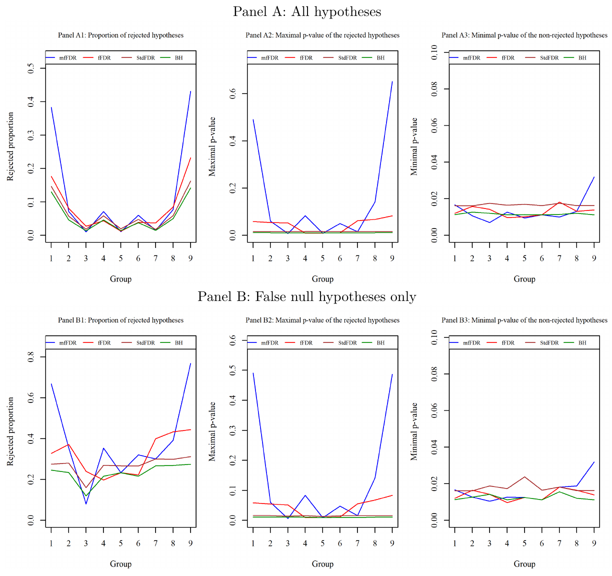
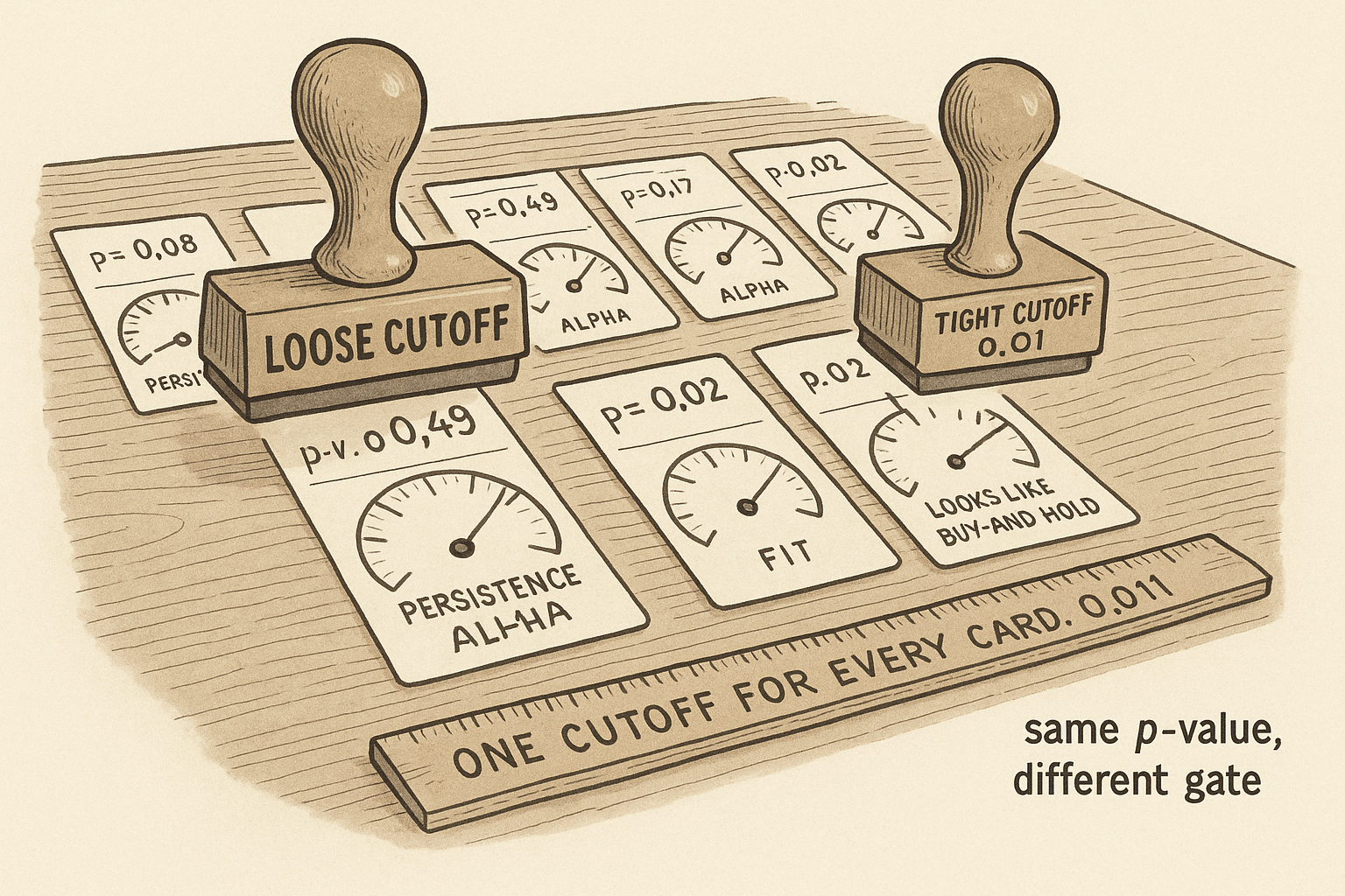
The paper reads that panel as a group-1 cutoff of 0.491 and a group-3 cutoff of 0.01. Benjamini-Hochberg sits near 0.011 and Storey's procedure near 0.016, the same number in every group. Inside group 1, one hypothesis with a p-value of 0.017 is refused while others with p-values up to 0.491 are kept, because the posterior uses the covariates together with the p-value. At the 20% target in their Monte Carlo, this two-covariate rule improves on the single-covariate rule by roughly 10% to 20% of the true alternatives. In the weak-signal design the largest gains are 57% against the single covariate, 62% against Storey, and 62% against Benjamini-Hochberg.
You reject on the q-value, an average of those posteriors
Sort the rules by the posterior null probability, smallest first. Walk down the list and stop at the largest set whose average posterior is still at or under the target. The q-value of a rule is that average for the set of every rule with a posterior no larger than its own. You reject the rule when the q-value is at or under the target. The empirical target is 20%, written 0.20.
$$ \hat q_i = \frac{1}{\# S_i}\sum_{k \in S_i}\hat r(p_k,z_k), \qquad S_i = \{k : \hat r(p_k,z_k) \le \hat r(p_i,z_i)\} $$
The set S is every rule at least as convincing as this one, ranked by the posterior. The q-value is their average posterior null probability. Four toy rules with posteriors 0.05, 0.12, 0.40, and 0.90, and a target of 0.20. The first q-value is 0.05. The second is (0.05+0.12)/2, which is 0.085. The third is (0.05+0.12+0.40)/3, which is 0.190. The fourth is (0.05+0.12+0.40+0.90)/4, which is 0.3675. You keep the first three and drop the fourth. The third rule has a posterior of 0.40 on its own, and it still enters, because the rules in front of it pull the average down to 0.190.
That is the sense in which a hard t-stat gate throws alpha away. The old article "Selection vs Diversification: Why |t|>3 Throws Away Alpha" makes the point for a portfolio: a cutoff that only keeps the loudest signals drops weak ones that diversify. Here the same idea is a moving p-value gate. In the simulation a p-value of 0.491 survives in a cell full of false nulls, and a p-value of 0.01 fails in a cell full of true nulls.
On the currencies, the extra keeps are large. Over 1973 to 2020, at the same 20% target, the common cutoff holds 1,530 Australian rules a month on average and the four-covariate screen holds 7,636. Japan is 2,145 against 8,282. I am against reading 7,636 as 7,636 independent discoveries. Moving-average rules are 12,870 of the 21,195 specifications, about 61% of the menu, and a 10-day average and a 15-day average are close to one trade. The netting step is what collapses them.
The position is the net signal, held for a month
Once the screen has fired, you add the signals and divide by the number of selected rules. Opposing rules cancel. The position you send is one number per currency, between -1 and +1.
$$ w = \frac{1}{N}\sum_{j \in \mathrm{selected}} S_j $$
N here is the count of selected rules, and S is each rule's signal in [-1, +1]. The paper's example: 100 selected rules, 30 long, 20 short, 50 flat. The sum of signals is 30 minus 20, which is +10. Divide by 100 and the position is 0.10, a 10% long in the foreign currency. If that currency's excess return over the next day is 1%, the book earns 0.10 times 1%, which is 10 basis points. A one-third signal from a triple moving average enters that same sum.
You form the book at the start of the month from the trailing 12 months, and you hold the weights for one month. Selection uses the pre-cost Sharpe. The held month is scored after costs. For a single currency the covariates are autocorrelation, buy-and-hold alpha, buy-and-hold beta, and buy-and-hold R-squared. For the pooled book you run the screen on every rule-currency pair together, and the benchmark inside alpha, beta, and R-squared is the equal-weighted basket of the 30 currencies. Capital is split equally across the selected rule-currency lines. Inside a currency you still net before you send the order. In 2011 to 2020 the screen selects 113,160 rules a month on average. After you net inside each pair, the order is one weight per currency. The 113,160 rules are the inputs to that sum.
The pooled book clears a Sharpe near one, then fades
Look at the orange bars. They are the net Sharpe of the pooled book. The rightmost pair is 2011 to 2020.
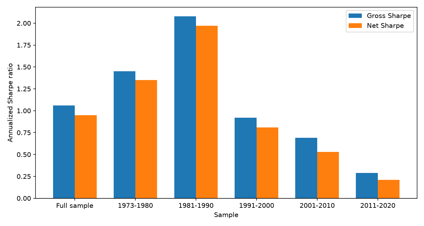
The full-sample gross Sharpe is 1.06 and the net Sharpe is 0.95. The 2011 to 2020 net Sharpe is 0.21. Across the 30 currencies, run one at a time, the average net Sharpe is 0.26 for the four-covariate screen, 0.18 when the four covariates are replaced by their first principal component, and 0.06 for a single cutoff, with a paired t-stat of 5.1 on the four-covariate average against that cutoff; Israel goes the other way, 0.73 on the single cutoff and 0.39 on the multivariate screen, Hungary and Poland are the two currencies where the multivariate net Sharpe is negative, and the pooled book's net Sharpe in the 1980s was 1.97.
The principal-component row is the result that justifies keeping four covariates. Crushing them into one index, and then running the single-covariate procedure on that index, lands on 0.18. The joint screen lands on 0.26. That gap is measured on the version that drops cross-product terms. It is four main effects against one index. The simulations, where the interaction is fit, are where Benjamini-Hochberg and Storey lose on power. The traded horse race is the single cutoff, the single covariate, the principal component, and the four-covariate screen.
Moving the target from 10% to 40% leaves the full-sample net Sharpe between 0.88 and 1.00. Sixteen of the thirty single-currency net Sharpes are statistically significant on the paper's own test. The average is the claim, and several of the country results are noise around it. Australia's multivariate net Sharpe is 0.14 with a p-value of 0.29.
Size the overlay to a few percent of volatility, and drop RSI
Their cost is one-third of the quoted one-month forward bid-ask spread, charged when the position changes. Where the forward quote is missing, developed currencies pay a fixed 5 basis points a trade in the 1970s, 4 in the 1980s, and 3 in the 1990s. Emerging currencies pay one-third of the average of the first 500 available bid-ask spreads, a constant, so the peso's cost does not widen on the day it gaps. I would replace that constant with the spread on the day you trade before believing an emerging-market line.
Full sample, the excess return is 3.80% and the net return is 3.40%, so the cost schedule removes 0.40 percentage points a year. Divide 3.80 by 1.06 and the gross book is a 3.58% volatility overlay. The one-way break-even cost, the fixed cost that takes the net Sharpe to zero, is 60 basis points. The paper does not print the turnover behind that 60. Divide the 3.80% gross return by 0.60% and you get 6.3 one-way trades a year if that cost is what wipes the gross book. Divide the 3.40% net return by 0.60% and you get 5.7 if the 60 basis points sits on top of their schedule. Either reading is a handful of turns a year, which is what netting does to a pile of overlapping rules. The last decade's break-even is 14 basis points, the net return is 0.63%, and 0.63 divided by 0.21 is 3.00% volatility. I am against levering that overlay up to a fully invested FX book.
The family split tells you which rules are paying for the turns. Run the same screen inside each family. Moving averages, the bulk of the menu, have a full-sample net Sharpe of 0.92 and a break-even of 71 basis points. Filters have a higher gross Sharpe, 1.26, and a break-even of 23 basis points, because they trade more. The relative-strength slice has a full-sample net Sharpe of -0.96, and it loses in every subperiod. I am against leaving it in the mix. The paper treats the selection rates as in-sample prevalence on the one-year window. Over the whole sample, 27% of rules are selected in a given month, 34% of moving averages, 13% of relative-strength rules. The rate falls from 36% in the 1970s and 1980s to 18% in 2011 to 2020.
The screen does move the book as the developed currencies go quiet. In 1973 to 1980 the largest share of selected rules is the yen, at 14.8%. In 2011 to 2020 it is the Argentine peso, at 10.1% of 113,160, about 11,400 rules a month. The paper reports that 30% of currencies still show a positive net Sharpe in that decade, and 41% of selected rules land in those currencies. The other 59% of the selected rules sit in currencies that lose money out of sample.
The regressions they run on the environment are thin, and one of them flips. A panel with a separate intercept per currency, of the annual portfolio return on a Scopus count of trading-technology papers per million people, has a coefficient of -0.007 and an adjusted R-squared of 0.028. Openness comes in negative as well, and the fit on the combined panel is 0.032. A monthly panel links higher aggregate volatility and higher illiquidity to higher returns, coefficients 0.010 and 0.029, and stock-market capitalization comes in at -0.021, with an adjusted R-squared of 0.030. Lag the same illiquidity measure and the coefficient flips to -0.020. I am against timing the book on either series. The after-cost edge shrank as the currencies got deeper, and what remains in the last decade is a low-volatility overlay concentrated in the thinner names, with a 14 basis point break-even.
What you run, if you run it, is the pooled screen. Trailing 12 months, positive-Sharpe rules only, four covariates kept separate, false-discovery target 0.20, q-value at or under that target, signals netted inside each pair, held for a month, sized to something like 3% to 4% annual volatility. Leave the relative-strength family out. Treat alpha as a summary of the same window that produced the Sharpe. And when the break-even on the live book is 14 basis points, you are one wide emerging-market day away from giving the decade back.
KEY POINTS
- Rescore the trailing 12 months and let autocorrelation, alpha, beta, and R-squared move the cutoff. At a 20% target the four-covariate screen keeps 7,636 Australian rules a month, against 1,530 for one cutoff.
- Reject on the q-value, the average posterior null probability of every rule you would keep with it. A target of 0.20 means that average stays at or under 0.20.
- Net the signals inside each currency and hold the weight for a month. The pooled book, 1973 to 2020, has a net Sharpe of 0.95.
- Keep the four covariates out of a single principal component. That compressed screen averages a net Sharpe of 0.18 across the 30 currencies.
- Do not lever 2011 to 2020. The pooled net Sharpe in that decade is 0.21.
References
- The Factor Zoo and the Multiple-Testing Reckoning
- Selection vs Diversification: Why |t|>3 Throws Away Alpha
- A Multivariate Covariate-Enhanced False Discovery Rate Method: Evidence from Technical Trading in Currency Markets (Filippou, Hsu, Ma, Sermpinis, and Taylor)
A note on AI. The ideas, research, analysis, and conclusions in this article are my own. I use AI tools to help with editing and wordsmithing, because English is not my first language, and I am not shy about that. AI-generated ideas and AI-assisted writing are not the same thing: the first is empty slop from a generic prompt, the second is a tool for communicating years of real research more clearly. Judge the work by its substance, not by whether software helped polish the prose.