3.57 Search Honestly: Metaheuristics, Plateaus and Diversity
Bitcoin rule search by differential evolution: report population diversity, stop at the geometric knee, and scale a linear Sharpe by the replication ratio.
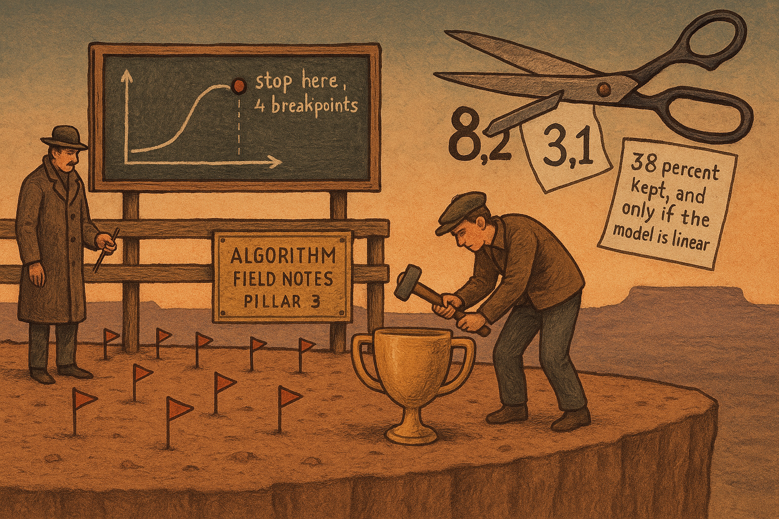
Hernández-Romo, Lemus-Romani, Vega, Becerra-Rozas and Romo tune a four-moving-average rule on 5-minute BTC/USDC, and they log how spread out the candidate population stays. After 1,000 generations, differential evolution is still spending 80 to 85 percent of its search on exploration. A population that never collapses has found a plateau of distant rules with similar average return, the same shape the old article "Collinearity in Parameter Sweeps: Plateaus, Not Peaks" found on a grid. Steiner's geometric knee decides how many kinks that plateau is allowed to have. The replication ratio in Jacquier, Muhle-Karbe and Mulligan is the fraction of a linear model's in-sample Sharpe that survives out of sample. Arakelian and coauthors supply the matching penalty on a rule search: the configuration ranked first in sample can rank below the median on the next window.
A window score is an average of eight overlapping backtests
The rule is a four-SMA crossover. SMA, the simple moving average, is the mean of the last N closes. One pair opens the long when the fast average crosses above the slow one. A second pair opens the short on the opposite cross. Take-profit and stop-loss are price multipliers that trail in your favor and freeze when price goes against you. One position at a time, 1x leverage, the whole account in the trade. That is eight knobs: four lookback lengths, each an integer from 5 to 200, and four multipliers. The long take-profit sits in 1.0 to 1.3, the long stop in 0.9 to 0.99, the short take-profit in 0.9 to 0.99, the short stop in 1.0 to 1.1. The search also penalizes any trade held longer than 5 days, which they write as 432,000 seconds. Five times 86,400 is 432,000, so that conversion is right.
They do not score a knob-setting on the whole history once. The training tape is BTC/USDC from 1 January 2020 through 31 December 2022, and each candidate has to earn its return on a rolling window. Let the price series have length T. Window k starts and ends at
$$ t^{(k)}_{\mathrm{start}} = 1 + (k-1)\, W_{\mathrm{step}}, \qquad t^{(k)}_{\mathrm{end}} = t^{(k)}_{\mathrm{start}} + W_{\mathrm{size}} - 1 $$
with the window kept only while the end index is still inside T. The start jumps forward by the step, and the end is the start plus the window length minus one, because both ends are included. Their study uses an 8-month window and a 4-month step. Count the training span as 36 months, so T = 36, the size is 8 and the step is 4. Window 1 runs from month 1 to month 8, January through August 2020, which is the example they print. Window 2 runs from month 5 to month 12, May through December 2020, also theirs. Window 8 runs from month 29 to month 36, May through December 2022. Window 9 would end at month 40, past the tape, so it is dropped. The paper never states the count. The dates they do state imply eight windows, and the overlap is (8 minus 4) divided by 8, which is one half. Four of those windows can be laid end to end without sharing a month. Eight is the number you average. Four is the stricter count of non-overlapping blocks, and that stricter count is mine, not theirs.
The fitness of a parameter vector x is the average window return,
$$ \mu(x) = \frac{1}{M} \sum_{j=1}^{M} r^{(j)}(x) $$
M is the number of windows that fit, and r to the j is the total return of the rule inside window j. The optimizer maximizes that average. Suppose the eight window returns are 0.40, 0.55, 0.20, 0.70, 0.10, 0.90, 0.30 and 0.45. The paper never prints the eight bitcoin window returns, so these are a worked example. The sum is 3.60, and 3.60 divided by 8 is 0.45. The search scores 45 percent, and the identity of the strong window is averaged away.
Two things follow before any optimizer is named. The fitness is average return. Sharpe and Sortino show up later as a report card, after the search has already ranked vectors by the thing in the card above. And a 5-minute bar is not an independent trial. The thing being estimated has about eight tries, four if you refuse the overlap.
Diversity is distance from the population centroid
Differential evolution (DE), the grey wolf optimizer (GWO), the whale optimization algorithm (WOA), and particle swarm optimization (PSO) each run a population of 50 vectors for 1,000 generations, and they repeat the whole run from 31 seeds. Hernández-Romo and coauthors then do the unusual thing: they publish the geometry of the population, using the diversity in their equation (22).
$$ \mathrm{Div} = \frac{1}{l \cdot n} \sum_{d=1}^{l} \sum_{i=1}^{n} \left| \bar{x}^{d} - x_{i}^{d} \right| $$
n is the population size, l is the number of knobs in each vector, x with subscript i is individual i, and the bar-x on dimension d is the mean of the population on that knob. The absolute value is how far that individual sits from the centroid on that knob. You average those distances over people and over knobs. The source writes an arrow over the centroid symbol; the sentence under the equation defines it as the mean. I use the mean.
Take four vectors in two dimensions: (0, 0), (0, 10), (10, 0), (10, 10). The centroid is (5, 5). On the first coordinate the absolute deviations are 5, 5, 5 and 5, which sum to 20. The second coordinate does the same. The double sum is 40. Here l is 2 and n is 4, so Div equals 40 divided by 8, which is 5. Move the same four points halfway in, to (2.5, 2.5), (2.5, 7.5), (7.5, 2.5) and (7.5, 7.5). The centroid is still (5, 5), the double sum falls to 20, and Div falls to 2.5. A population sitting on one vector has Div equal to 0.
They turn that level into an exploration share and an exploitation share, normalized by the largest diversity the run itself recorded:
$$ \mathrm{XPL\%} = \frac{\mathrm{Div}}{\mathrm{Div}_{\max}} \cdot 100, \qquad \mathrm{XPT\%} = \frac{\left| \mathrm{Div} - \mathrm{Div}_{\max} \right|}{\mathrm{Div}_{\max}} \cdot 100 $$
XPL percent is exploration, XPT percent is exploitation. Div max is the highest diversity seen in that run, so the two shares describe the run relative to its own widest moment. While Div stays at or below that maximum, the absolute value is Div max minus Div, and the two percentages add to 100. In the toy, Div max is 5 and the halfway population has Div 2.5, so exploration is 50 and exploitation is 50.
XPL percent is a fraction of the widest dispersion that same run recorded, so a cloud jittering in place at a wide dispersion scores high exploration for all 1,000 generations, and a cloud that falls onto one basin scores low. The trace answers whether the population collapsed. The fitness still has to say whether the place it sits is any good.
The knee is the breakpoint count farthest from the chord
A plateau still has a complexity choice. Steiner fits a connected piecewise-linear trend to an index, one new slope-change per breakpoint, and the in-sample R-squared keeps rising as breakpoints are added. R-squared here is one minus the residual sum of squares over the total sum of squares. The fit at 15 breakpoints is closer than the fit at 4, and a search that maximizes R-squared will take the 15. The geometric knee is the stop.
$$ R^{2}(K) = 1 - \frac{\mathrm{RSS}(K)}{\mathrm{SS}_{\mathrm{tot}}} $$
RSS(K) is the residual sum of squares with K breakpoints, and SS tot is the sum of squared deviations from the sample mean of the series. If the residuals sum to 80 and the series sums to 100 in squared deviation, R-squared is 1 minus 0.80, which is 0.20. That is a legal input to the next card. The old article "Piecewise-Linear Regime Identification (Interpretable, No Black Box)" reads the slopes as bullish, flat, and bearish regimes. The object here is only where you stop adding slopes.
Fit K from 0 out to some maximum. Plot R-squared against K. Draw the straight chord from the first point to the last. For each interior K, measure the perpendicular distance to that chord and keep the K with the largest distance.
$$ d_{k} = \frac{\left| v_{x}\, (R^{2}(k) - R^{2}(0)) - v_{y}\, (k - 0) \right|}{\sqrt{v_{x}^{2} + v_{y}^{2}}}, \qquad k^{*} = \arg\max_{k} d_{k} $$
The vector v runs from the K = 0 point to the K = K max point, so its components are the change in breakpoint count and the change in R-squared. The numerator is the absolute value of the two-dimensional cross product between v and the vector from the start point to the candidate. Dividing by the length of v converts that area into a distance. The knee k star is the candidate farthest off the chord. Past it, another breakpoint buys a thin slice of in-sample fit.
Use a curve small enough to recompute. Let R-squared at breakpoint counts 0 through 6 be 0.20, 0.55, 0.70, 0.75, 0.78, 0.79, 0.80. The chord runs from (0, 0.20) to (6, 0.80), so v is (6, 0.60) and its length is the square root of 36.36, which is 6.030. At 2 breakpoints the point sits at (2, 0.70). The cross product is 6 times 0.50 minus 0.60 times 2, which is 1.80. The distance is 1.80 divided by 6.030, which is 0.299. The same arithmetic at 1, 3, 4 and 5 breakpoints gives 0.249, 0.249, 0.179 and 0.090. The maximum is at 2. This curve is a worked example, not Steiner's index.
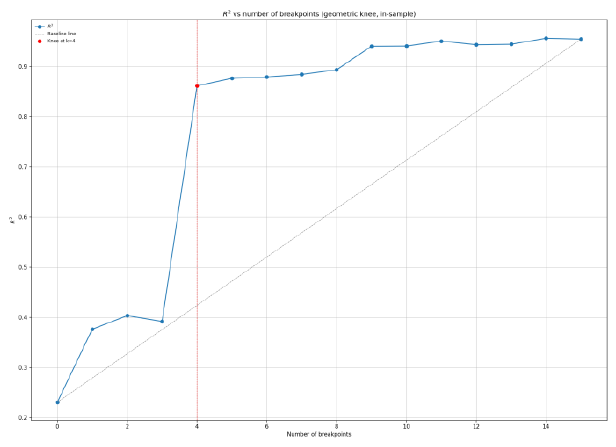
On the Swiss Leaders Index the red marker sits at 4 breakpoints. The curve has already done its steep climb, and further breakpoints add a shallow slope. You keep 4. You do not keep 15 because 15 wins the in-sample R-squared. The same stop applies to a rule search: if you are choosing how many moving averages, filters, or exits to hand the optimizer, plot the score against that count and take the knee. The eight-knob SMA rule in the bitcoin study never received this treatment. Eight knobs were fixed in advance, then optimized.
The replication ratio is out-of-sample Sharpe over in-sample Sharpe
Diversity says the search found a cloud. The knee says which cloud size you allow. Neither one tells you the Sharpe you should expect next month. That number is the replication ratio in the old article "The Real IS→OOS Sharpe Haircut (Closed Form, Not "50%")", and Jacquier, Muhle-Karbe and Mulligan derive it for a specific machine: a linear forecast, ordinary least squares, signals that are independent across time, a Markowitz book that already knows the residual covariance.
One asset, one signal, no intercept, signal scaled so its variance matches the residual variance. Write beta for the true coefficient and T_1 for the number of in-sample steps. Their equation (3.3) prints the subscripts in a compressed way, T with a subscript 1-2 and T with a subscript 1+2. Those are T_1 minus 2 and T_1 plus 2. Expanded, the expected in-sample Sharpe and the expected out-of-sample Sharpe are
$$ \mathrm{SR}_{\mathrm{EIS}} = \frac{\beta^{2} + \frac{1}{T_{1}}}{\sqrt{2\beta^{4} + \left(1 + \frac{15}{T_{1}-2} - \frac{2}{T_{1}}\right)\beta^{2} + \frac{4}{T_{1}} - \frac{3}{T_{1}+2} - \frac{1}{T_{1}^{2}}}} $$$$ \mathrm{SR}_{\mathrm{EOOS}} = \frac{\beta^{2}}{\sqrt{2\beta^{4} + \left(1 + \frac{2}{T_{1}-2}\right)\beta^{2} + \frac{1}{T_{1}-2}}} $$
The replication ratio is the second divided by the first. Both Sharpes are per time step, mean PnL over the standard deviation of PnL. Multiply by the square root of 252 when you want the usual annual figure under independent days, and scale both legs together. The ratio is unchanged by that scaling.
The numerator is the part to stare at. In the general case of their Proposition 3.1, with m assets and p signals, centred and standardized, the expected in-sample mean PnL equals the trace of Gamma plus p times m over T_1. The expected out-of-sample mean PnL equals the trace of Gamma and nothing else. Gamma is beta transpose times the inverse residual covariance times beta. The trace is the real linear edge. The added term p m over T_1 is fit to the noise in the training window, and it is absent once the window moves. With one asset and one signal the added term is 1 over T_1, which is why the in-sample numerator is beta squared plus 1 over T_1 and the out-of-sample numerator is beta squared alone.
Put beta at 0. There is no signal. Set T_1 to 252, one year of daily steps. The in-sample numerator is 1/252, which is 0.003968. The quantity inside the square root collapses to 4/252 minus 3/254 minus 1 over 252 squared, which is 0.004046. Its square root is 0.06361. Divide 0.003968 by 0.06361 and the expected in-sample Sharpe is 0.0624 per step. Times the square root of 252, that is 0.99 annualized. The out-of-sample numerator is 0, so the out-of-sample Sharpe is 0 and the replication ratio is 0. A single useless coefficient, on a single asset, for a single year, prints an in-sample annualized Sharpe near 1 and then nothing. A 50 percent haircut would still leave you a fake 0.5. The ratio here leaves you zero.
Now give the signal a pulse, beta squared equal to 0.01, same T_1 of 252. The true per-step Sharpe, before any estimation, is 0.0990. The formulas above give an expected in-sample Sharpe of 0.1149 and an expected out-of-sample Sharpe of 0.0837. The replication ratio is 0.728. The ratio is 0.728. The in-sample figure was already above the truth, 0.1149 against 0.0990. The true per-step Sharpe is 0.01 divided by the square root of 0.0102, which is 0.0990.
The commodity case is where the parameter count starts to hurt. Twelve futures, three momentum horizons each plus an intercept, so p equals 3 times 12 plus 1, which is 37 regressors. Coefficients equal 37 times 12, which is 444. They simulate 252 days times 10 years in sample. The wide regression keeps a replication ratio they state as 38 percent, with an in-sample Sharpe of 8.2 and an out-of-sample Sharpe of 3.1. Dividing those two printed Sharpes gives 3.1/8.2 = 0.378, so the 38 percent matches. Forcing one weight per horizon across all twelve markets cuts the coefficient count from 444 to 3. They state that panel's replication ratio as 70 percent, from an in-sample Sharpe of 0.9 and an out-of-sample Sharpe of 0.6. Dividing those two gives 0.6/0.9 = 0.67, which is under the 70 percent they print. I keep both the 70 and the 0.67. The source may be rounding a distribution of ratios, not the ratio of the two rounded Sharpes. On that simulation the wide model still has the higher out-of-sample level, 3.1 against 0.6, because the data were generated by the wide model. The constraint throws away real coefficients. The ratio improves. The level falls.
On the real equity-premium predictors the level flips. The panel's out-of-sample Sharpe is 0.5 against the wide model's 0.3, with in-sample Sharpes of 0.7 and 3.6. They call the ratios 68 percent and 9 percent. The quotients of the printed Sharpes are 0.5/0.7 = 0.71 and 0.3/3.6 = 0.083. Those sit near 68 percent and 9 percent, and they disagree with them. The stated ratio may be a distribution of ratios, while the Sharpes are rounded point estimates. I keep the source's 68 and 9. The introduction's Figure 1 puts a ten-year commodity backtest at 30 percent, and Section 5 puts the ten-year full regression at 38 percent. The paper does not say which specification the 30 percent used. I quote both and I do not average them.
These formulas take a linear regression as their input. Here p is a column count, and T_1 is a count of return steps the regression sees one at a time. A path-dependent stop has no column in that design matrix. Counted on the bitcoin training design anyway, there are eight windows and eight knobs. The variance terms divide by T_1 minus p minus 1. Eight minus eight minus one is negative, so the formula is outside its domain. Report that fact. Eight knobs on eight overlapping windows, four if the overlap is stripped out, never entered the region where this haircut is defined.
The in-sample winner can rank below the median
Arakelian and coauthors write the selection problem down. You have N strategies, you rank them in sample, and you keep the one whose in-sample rank equals N, their label for the winner. The probability of backtest overfitting, PBO, is the probability that this winner's out-of-sample rank falls below N/2, averaged over which strategy won:
$$ \mathrm{PBO} = \sum_{n=1}^{N} \mathrm{Prob}\!\left( \bar{r}_{n} < N/2 \,\big|\, r \in \Omega_{n}^{*} \right) \, \mathrm{Prob}\!\left( r \in \Omega_{n}^{*} \right) $$
The bar-r is the out-of-sample rank, with larger meaning better, and Omega star n is the set of rankings in which strategy n won in sample. For a search that has already produced one winner, the sum collapses to the conditional probability that this winner's out-of-sample rank is below N/2.
The bitcoin study keeps the best of 31 seeds when it wants a single configuration. Set N to 31. If the out-of-sample rank of the in-sample winner is uniform on 1 through 31, the ranks strictly below 15.5 are 1 through 15. That is 15/31, or 0.48. Under pure noise you are essentially flipping a coin on whether the seed you are about to publish sits in the bottom half. The sentence above their formula uses a different cutoff: it calls the selection overfit when the expected out-of-sample rank is at or below N/2. A uniform rank on 1 through 31 has expectation 16, and 16 is above 15.5, so that sentence does not flag the same case the probability flags. I keep both cutoffs as printed. The action does not depend on the boundary. You publish the median seed across the 31 runs, and you publish the diversity trace. The maximum seed is a draw from the plateau.
Differential evolution stays spread out; the swarms fall in
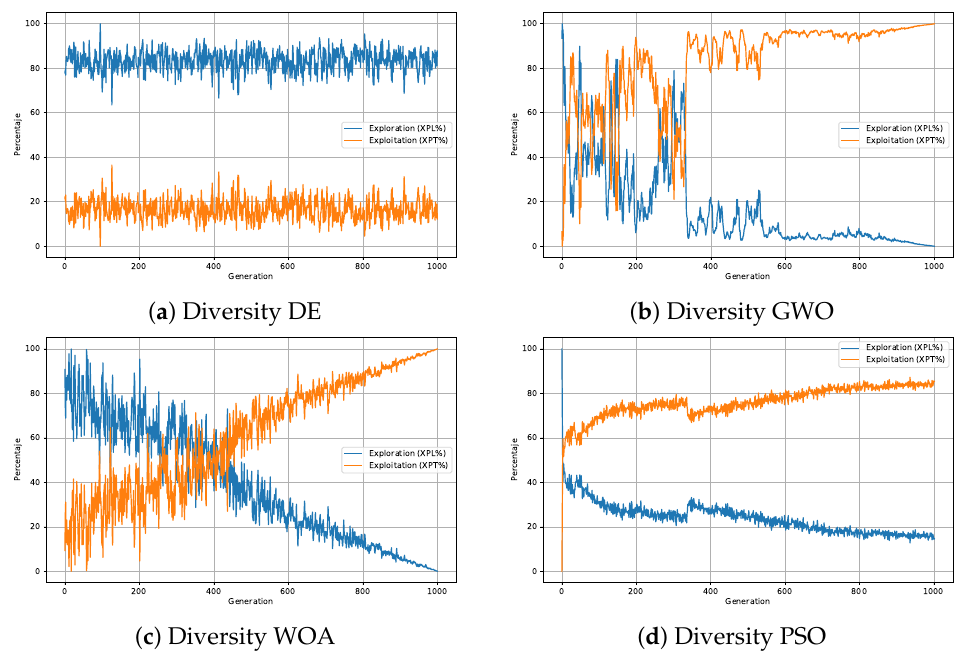
Look at the blue exploration line in panel (a). It stays inside a band near 80 to 85 percent from the first generation through generation 1,000. The orange exploitation line is the remainder, near 15 to 20 percent. Panels (b) and (d), grey wolf and particle swarm, do the textbook thing the diversity literature expects: exploration dies and exploitation takes the population. The paper puts that collapse near generation 350 for grey wolf and particle swarm. Whale, panel (c), hands off smoothly, exploration falling and exploitation rising across the whole run.
DE's average annualized return across seeds is 107.36 percent, and the average annualized volatility on that same column is 108.85 percent. The best DE row in the later table prints a Sharpe of 0.977, equal to 108.86 divided by 111.42, which rounds to 0.98. WOA, PSO and GWO average 92.05, 73.47 and 61.80 percent annualized. The single best validation run is WOA at 120.28 percent, with a Sortino of 3.95 (return over downside deviation), a profit factor of 5.06 (gross profit over gross loss) and a maximum drawdown of minus 28.66 percent. Table 5's "best" DE return is 119.62 percent and the later best-execution table prints 108.86 percent for DE; PSO moves from 121.48 to 110.84, WOA from 118.15 to 120.28, and GWO matches at 116.79. The paper does not reconcile the three that move. I quote 107.36 as the across-seed average, because that is the column tied to the objective, and I do not pick a best-run return from a pair of tables that disagree.
The annualized figure itself uses their equation (20). Total return r is ending equity over starting equity, minus one. The annualized return compounds that by 365 over d, where d is the number of days in the window. The sentence above the formula says the dataset has a 356-day trading year, and the exponent uses 365. On an illustration, a 50 percent window return over the 244 calendar days from 1 January through 31 August 2020, the 365-day exponent gives 83.41 percent and the 356-day exponent gives 80.68 percent. I keep 365, because that is the formula they printed, and the 356 is a stray sentence. The 244 days and the 50 percent are mine, so you can see the gap. They are not a bitcoin window return.
DE winning the average-return column is the objective doing what it was told. WOA takes the best-run Sortino, and PSO prints the highest best-run Sharpe at 1.086. Which models survive depends on which loss you rank by, which is Arakelian and coauthors' evaluation point. The prose of the Wilcoxon rank-sum test, which ranks the seeds and compares those ranks, says DE beats WOA on mean return at p under 0.01, and beats GWO on the best validation return at p equal to 0.02. Several cells of the printed table show a greater-than sign, as in p greater than 0.001, on comparisons the note marks as significant. A significance call needs the inequality the other way. I leave the table as printed and follow the prose. The greater-than signs look like a transcription error.
Grey wolf and particle swarm collapse, so one seed can print an extreme best case and the next seed a bad one. Differential evolution stays dispersed. Hernández-Romo and coauthors read that as several basins of similar fitness occupied at once: the scores have bunched, and the vectors are still far apart. That is a plateau. The best vector in the log is one occupant of it. The best DE configuration they describe in words holds trades for 39 days on average, while the search penalizes holds past 5 days. Either the penalty left that point alone, or the 39 days are measured on the January 2023 to March 2025 validation slice, where the penalty was not reapplied.
At the desk, the estimate is a median, a trace, and a haircut
Run the search after the rule exists. The old article "Optimization Comes After Testing, Not Before" is the order of operations, and this study follows it only halfway: the four-SMA skeleton is fixed, and then eight knobs plus the optimizer's own controls are still free. DE's difference scale F ranges from 0.4 to 0.8, and CR, the fraction of coordinates taken from the trial vector, ranges from 0.5 to 0.9. That is another search wrapped around the search.
Score every candidate on the rolling windows and store the return of each seed. The number you keep is the median across the 31 seeds. Store the diversity trace. If the exploration share is still near 80 percent at generation 1,000, write "plateau" on the report and keep a handful of distant vectors whose window-average returns sit near that median. If you are choosing how many indicators or breakpoints to admit, stop at the knee of the score-versus-count curve, the way the Swiss Leaders fit stops at 4.
Apply the replication ratio only to a linear forecast, with p, m and T_1 counted the way Proposition 3.1 counts them. A ten-year, twelve-market momentum regression with 444 coefficients is the scale they computed: 38 percent kept in the simulation where the wide model is true, and on the real equity-premium set the three-coefficient panel has the higher out-of-sample Sharpe, 0.5 against 0.3. Leave the four-SMA rule out of that formula. Eight knobs on eight windows sit where T_1 minus p minus 1 is negative. That sentence is the estimate.
Costs they did include: 0.05 percent commission per fill, copied from Binance, and a single unlevered position. The best DE run they describe takes 20 trades. If each trade opens and closes, that is 40 fills, and 40 times 0.0005 is 0.02, two percentage points of commission over the validation window. Two points leave a triple-digit annualized return standing. The paper prints no slippage figure separate from that commission, and no funding charge on the short. The book is in the market almost continuously, on 5-minute bitcoin. You add both before you set the result next to buy and hold.
Buy and hold over the validation window, January 2023 through March 2025, is printed as 397.93 percent. That is a cumulative number on a bullish slice of a bit more than two years. The strategy figures next to it are annualized. The paper does not print the strategy's cumulative return on that same slice, so I will not invent the conversion. I am against reading that across-seed average as a return you should expect. The fitness was that same average, the diversity trace stayed on a plateau, and eight knobs on eight windows sit outside the replication ratio.
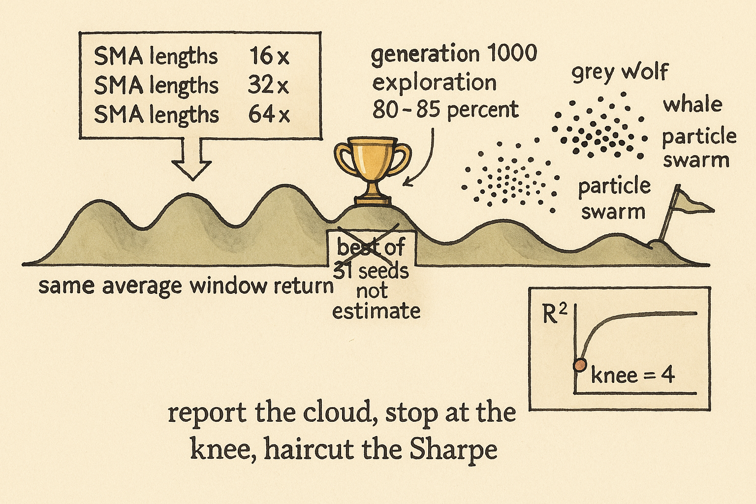
KEY POINTS
- Score each parameter vector on a rolling window and average the window returns. An 8-month window and a 4-month step on the 2020 to 2022 tape give eight windows, and four of them do not overlap.
- Track diversity. Differential evolution's exploration share stays at 80 to 85 percent through generation 1,000, so the population never collapsed onto one vector.
- Stop adding breakpoints at the geometric knee. On Steiner's Swiss Leaders fit the marker is at 4 breakpoints; on the worked curve the farthest point is at 2.
- Multiply an in-sample Sharpe by the replication ratio only for a linear forecast. With no signal, one coefficient and 252 days, the in-sample annualized Sharpe is about 0.99 and the out-of-sample Sharpe is 0.
- Publish the median of the 31 seeds and the diversity trace. Twenty round-trip trades at 0.05 percent a fill cost 2 percent in commission. The across-seed average the search was fit to is 107.36 percent annualized.
References
- Collinearity in Parameter Sweeps: Plateaus, Not Peaks
- Piecewise-Linear Regime Identification (Interpretable, No Black Box)
- The Real IS→OOS Sharpe Haircut (Closed Form, Not "50%")
- Optimization Comes After Testing, Not Before
- A Piecewise-Linear Model For Market Regime Identification
- In-Sample and Out-of-Sample Sharpe Ratios for Linear Predictive Models
- A discussion paper for possible approaches to building a statistically valid backtesting framework
- Robust Metaheuristic Optimization for Algorithmic Trading: A Comparative Study of Optimization Techniques
A note on AI. The ideas, research, analysis, and conclusions in this article are my own. I use AI tools to help with editing and wordsmithing, because English is not my first language, and I am not shy about that. AI-generated ideas and AI-assisted writing are not the same thing: the first is empty slop from a generic prompt, the second is a tool for communicating years of real research more clearly. Judge the work by its substance, not by whether software helped polish the prose.