7.6 The Math Stack, Extended: Ridge, Linear Models, and the Stats Canon
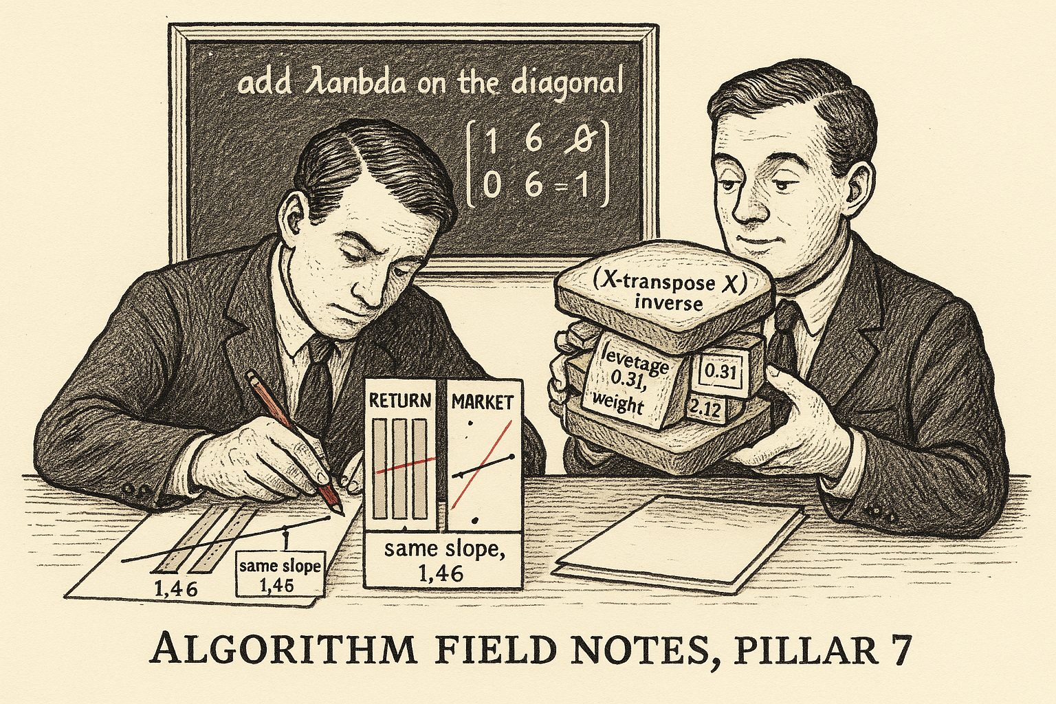
Ridge regression adds lambda on the diagonal of X-transpose X before inverting. Eigenvalue 10 keeps 10/11 of its least-squares weight at lambda 1; a zero eigenvalue keeps none.
Ordinary least squares asks you to invert X-transpose X. On the four-row design in van Wieringen's ridge notes the first column is the sum of the other two, so that matrix has a zero eigenvalue and the inverse does not exist. Ridge adds a penalty lambda on the diagonal and the inverse comes back. At lambda equal to 10 the smallest of the three coefficients is 0.002. That closed form is the estimator under the L2 rate in the old article "The Mathematics of Machine Learning, for Traders". The notes below are the algebra you type, and they stay out of the P&L column.
A zero eigenvalue means there is no least-squares coefficient
The linear fit you already run is ordinary least squares. With a design matrix X, one row per day and one column per feature, and a response y, the coefficient vector minimizes the sum of squared residuals. Van Wieringen writes the normal equation as X-transpose X times beta equals X-transpose y, and the solution, when the inverse exists, is the maximum-likelihood estimator under Gaussian errors. Ding and Rahaman print the same minimizer.
$$ \hat{\beta} = (X^{\top} X)^{-1} X^{\top} y $$
X-transpose X is the p by p matrix of unnormalized feature inner products. You invert it and multiply by X-transpose y, which is the inner product of each feature with the response. The result is the unique coefficient vector only when that p by p matrix has full rank.
Van Wieringen's Example 1.3 is small enough to invert by hand and singular on purpose:
$$ X = \begin{pmatrix} 1 & -1 & 2 \\ 1 & 0 & 1 \\ 1 & 2 & -1 \\ 1 & 1 & 0 \end{pmatrix}, \qquad X^{\top} X = \begin{pmatrix} 4 & 2 & 2 \\ 2 & 6 & -4 \\ 2 & -4 & 6 \end{pmatrix}. $$
Column 1 equals column 2 plus column 3 on every row, so the rank is 2 and the determinant is 0. The eigenvalues of X-transpose X are 10, 6, and 0. A zero eigenvalue means a whole line of coefficient vectors fit the columns equally well: add any constant c to the first coefficient and subtract c from the other two, and X beta does not move, because X times (1, -1, -1) is the zero vector. There is no unique least-squares beta. The response he pairs with this X is y = (1.3, -0.5, 2.6, 0.9). You still cannot quote an OLS coefficient.
The same blow-up shows up before the eigenvalue hits exactly zero. In his flotillin illustration two probes correlate at 0.91, and their standard errors come out 0.38 and 0.30 against 0.06 on a probe whose correlations with the others stay under 0.20. The regression R-squared is 0.05. Collinearity spends the precision on deciding which column gets the credit. A pair of features you built from the same price path does this to a return regression.
Lambda on the diagonal is the ridge estimator
Hoerl and Kennard's fix, as van Wieringen states it in Definition 1.2, replaces X-transpose X with X-transpose X plus lambda times the identity, for lambda at least 0.
$$ \hat{\beta}(\lambda) = (X^{\top} X + \lambda I)^{-1} X^{\top} y $$
You add lambda to every diagonal entry, then invert, then multiply by X-transpose y. The added matrix is positive definite for lambda above 0, so the sum is invertible even when X-transpose X is not. On the four-row design at lambda equal to 1 the matrix he prints is
$$ X^{\top} X + I = \begin{pmatrix} 5 & 2 & 2 \\ 2 & 7 & -4 \\ 2 & -4 & 7 \end{pmatrix}, $$
with eigenvalues 11, 7, and 1. The zero is gone. Solving against y gives beta-hat of 0.614, 0.548, and 0.066. At lambda equal to 10 the same solve gives 0.269, 0.267, and 0.002. His notes print those triples to three decimals; recomputing the linear system matches.
The spectral form in his section 1.3 says what happened to each direction. If nu is an eigenvalue of X-transpose X, ridge multiplies that direction's least-squares contribution by a weight
$$ \frac{\nu}{\nu + \lambda}. $$
A strong direction, large nu, keeps almost all of its weight. A weak direction keeps little. A zero eigenvalue keeps none, which is why the null-space coefficient dies instead of wandering off to infinity. On this design at lambda equal to 1 the weights are 10/11, 6/7, and 0/1, that is 0.91, 0.86, and 0. The effective number of parameters is the sum of those weights, his degrees-of-freedom trace:
$$ \mathrm{df}(\lambda) = \sum_{j} \frac{\nu_j}{\nu_j + \lambda}. $$
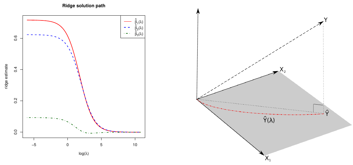
Three columns spend 1.77 degrees of freedom at lambda equal to 1, and 0.875 at lambda equal to 10 (10/20 plus 6/16 plus 0). As lambda goes to infinity the trace goes to 0 and every coefficient goes to 0. The left panel of his solution path is that decay. The right panel is the geometric cost: the ridge fitted vector is not the orthogonal projection of y onto the columns, so the ridge residual is not perpendicular to the fit. You bought an invertible system and gave up the exact least-squares projection.
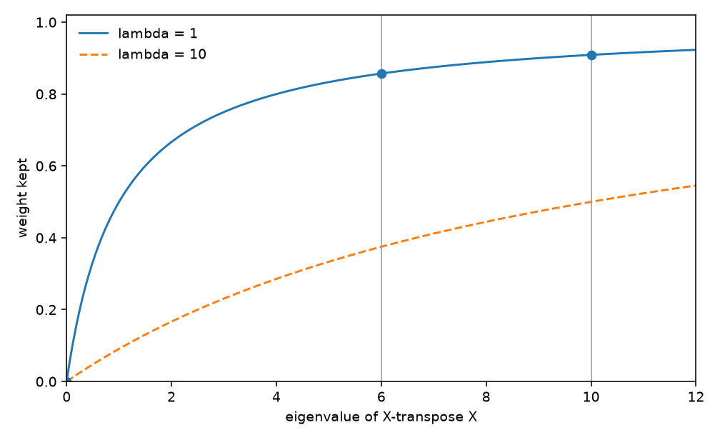
When the columns are orthonormal, X-transpose X equals the identity and every eigenvalue is 1, so the weight is 1 over 1 plus lambda. His Example 1.4:
$$ \hat{\beta}(\lambda) = \frac{1}{1+\lambda}\,\hat{\beta}. $$
An OLS coefficient of 0.40 becomes 0.20 at lambda equal to 1. Expectation moves with it. In general, with X treated as fixed,
$$ \mathbb{E}[\hat{\beta}(\lambda)] = (X^{\top} X + \lambda I)^{-1} X^{\top} X \, \beta = \beta - \lambda (X^{\top} X + \lambda I)^{-1} \beta. $$
The estimator is biased for any lambda above 0. Take four rows with columns (1, 0), (0, 1), (1, 1), (1, -1). The columns are orthogonal and X-transpose X equals 3 times the identity. At lambda equal to 1 the weight is 3/4. A true coefficient pair of 0.40 and -0.20 has expectation 0.30 and -0.15. You pulled each coefficient a quarter of the way to zero, on purpose, to cut variance. That trade is the content of the U-shaped error in the old article "The Mathematics of Machine Learning, for Traders". The rate there says what you pay. This is the vector you compute.
Toomet writes the same estimator as a penalized loss. Minimize residual sum of squares plus lambda times a penalty, and at lambda equal to 0 you are back at OLS.
$$ \min_{\beta}\ (y - X\beta)^{\top}(y - X\beta) + \lambda \, \beta^{\top} W \beta $$
W is a diagonal matrix of feature weights. He puts a 0 in the intercept position and 1 on every slope, so the penalty does not shrink the mean. Van Wieringen's Definition 1.2 uses lambda times the identity, which does penalize an intercept if you left a column of ones in X. On 100 rows, a mean of 0.001, lambda equal to 100: OLS returns 0.001, and penalizing the intercept returns 0.1 over 200, which is 0.0005. You halved the average return. For a return regression, center y and the features and drop the intercept, or zero that diagonal entry the way Toomet's W does.
His scalar line for the same penalty sums beta-sub-j squared on an index i running from 1 to n. Implemented literally, that multiplies the penalty by the sample size and penalizes a single coefficient. Use the matrix penalty. The closed form is
$$ \hat{\beta}(\lambda) = (X^{\top} X + \lambda W)^{-1} X^{\top} y. $$
With W equal to the identity on the slopes and zero on the intercept, this is Definition 1.2 on the slopes only.
Scale the columns before you penalize. A slope of 0.02 on a decimal return is a slope of 0.0002 on a percent return, the same economic bet. The squared penalty charges 0.0004 in the first unit and 0.00000004 in the second, a ratio of 10,000. Toomet's warning is the mile-versus-millimeter version of this. Standardize, or the penalty will crush whichever feature you happened to measure in small units.
When you have more features than days, do not invert the p by p matrix. Van Wieringen's section 1.7 points at a microarray with p equal to 40,000 and n equal to 100 and reduces the work through the singular value decomposition. He does not print the dual identity, which is the same reduction in one line:
$$ \hat{\beta}(\lambda) = X^{\top} (X X^{\top} + \lambda I_n)^{-1} y. $$
The matrix inside is n by n. On his microarray that is 100 by 100, not 40,000 by 40,000. The two expressions agree. On a random 5 by 8 check the largest absolute difference is under 10 to the minus 15.
The coefficient you quote is a regression of residuals on residuals
Ding's Theorem 7.1, the Frisch-Waugh-Lovell theorem, is how you read one slope in a regression that also contains controls. Split X into controls X1 (k columns, including the intercept if you have one) and the feature you care about, X2 (l columns). Let H1 be the hat matrix of the controls, X1 times (X1-transpose X1) inverse times X1-transpose. Residualize:
$$ \tilde{X}_2 = (I - H_1) X_2, \qquad \tilde{y} = (I - H_1) y, \qquad \hat{\beta}_2 = (\tilde{X}_2^{\top} \tilde{X}_2)^{-1} \tilde{X}_2^{\top} \tilde{y}. $$
Beta-2 from the long regression equals the OLS slope of the residualized response on the residualized feature. His equation (7.3) skips residualizing y and still recovers the coefficient, because the controls are orthogonal to X-tilde-2. Equation (7.4), the one above, residualizes both. Corollary 7.1 says the residual vector matches the full regression only in that second case.
Eight rows, so you can recompute it. Controls are an intercept and x1 = 1 through 8. The feature is x2 = (2, 1, 4, 3, 7, 5, 8, 6). The response is 0.4 plus 0.3 times x1 plus 1.5 times x2, plus the errors (0.2, -0.4, 0.1, 0.3, -0.2, 0.5, -0.1, 0). That produces
y = (3.9, 2.1, 7.4, 6.4, 12.2, 10.2, 14.4, 11.8).
The long regression, three coefficients, estimates the x2 slope at 1.458. Residualize y and x2 on the intercept and x1. The residual sum of products is 18.717 and the residual sum of squares of x2 is 12.833. Divide: 18.717 / 12.833 = 1.458. Regressing raw y on residualized x2, his form (7.3), gives the same slope. The residuals match the long regression to machine precision only when you residualized y as well. Residualize only the feature and the slope is still right, and the residual vector is a different object. If you then build a standard error or a trading residual from that second vector, you are not holding the full-model residual.
The algebra is not an experiment. Ding says so under Theorem 7.1: nothing in the projection holds the controls constant in the world. You removed the linear part of the controls from the feature. A coefficient you read as "the signal, after the market" means that, and only that.
The standard error does not come along for free. Theorem 7.2: if the long regression uses n minus k minus l degrees of freedom and the partial regression uses n minus l, the homoskedastic covariance estimates satisfy
$$ (n - k - l)\, \hat{V} = (n - l)\, \tilde{V}. $$
On these eight rows, k equals 2 and l equals 1, so the honest divisor is 5 and the partial regression's divisor is 7. The long-regression standard error on the x2 slope is 0.093. The partial regression's homoskedastic standard error is 0.079. The ratio is the square root of 5/7, and 0.079 times the square root of 7/5 (1.18) recovers 0.093. Quote the partial standard error raw and you understate the uncertainty, because you forgot the controls you already fitted. The Eicker-Huber-White covariance, HC0, matches across the two regressions with no degrees-of-freedom patch: both print 0.070 on this draw. Ding is explicit that the match is for that original sandwich and breaks for the modified versions HC1 through HC4.
The standard error puts each squared residual in the middle
Under heteroskedasticity the OLS coefficient is still consistent. The usual standard error, sigma-hat squared times the diagonal of (X-transpose X) inverse, is not. Ding's sandwich, the Eicker-Huber-White covariance, replaces the single sigma-hat squared with the squared residuals:
$$ \hat{V}_{\mathrm{EHW}} = (X^{\top} X)^{-1} (X^{\top} \hat{\Omega} X) (X^{\top} X)^{-1}, \qquad \hat{\Omega} = \mathrm{diag}(\hat{\varepsilon}_1^2, \ldots, \hat{\varepsilon}_n^2). $$
The two outer matrices are the bread. The middle is the meat: each row contributes its own squared residual times the outer product of its feature row. Rahaman prints the same estimator as HC0. Classical standard errors are the special case where every squared residual is replaced by one pooled variance.
A line through the origin, x from 1 to 8, true slope 0.5, errors (0.1, -0.1, 0.15, -0.05, 1.6, -1.4, 2.0, -1.8). The inner product x-transpose x equals 204 and x-transpose y equals 101.35, so the slope is 101.35 / 204 = 0.497. Residual sum of squares is 11.80. The classical standard error, dividing by n minus 1, is 0.091. The HC0 standard error is 0.114, which is 1.25 times the classical 0.091, because the big residuals sit on the large x values and the meat notices.
HC1 multiplies that covariance by n over n minus p. Ding defines it as a finite-sample inflation of HC0; Rahaman writes the same factor.
$$ \hat{V}_{\mathrm{HC1}} = \frac{n}{n-p}\, \hat{V}_{\mathrm{HC0}}. $$
Here p equals 1, so the factor is the square root of 8/7 on the standard error, and 0.114 becomes 0.121. On a year of daily rows with six coefficients the factor n over n minus p is 252/246, about 1.02. HC1 rescales the HC0 covariance. The heteroskedasticity is already in the meat.
HC3 divides each squared residual by (1 minus the leverage) squared before it enters the meat. Leverage of row i is the diagonal of the hat matrix, h-sub-ii equals x-sub-i transpose times (X-transpose X) inverse times x-sub-i. Through the origin that is x-sub-i squared over x-transpose x.
$$ \hat{V}_{\mathrm{HC3}} = (X^{\top} X)^{-1} \left( \sum_{i=1}^{n} \frac{\hat{\varepsilon}_i^2}{(1-h_{ii})^2} x_i x_i^{\top} \right) (X^{\top} X)^{-1}. $$
On this line the last row has leverage 64/204 = 0.314. The HC3 weight is 1 over (1 minus 0.314) squared, which is 2.12. The HC3 standard error comes out 0.152, against 0.091 classical and 0.114 for HC0. Rahaman's review recommends HC3 for a typical financial cross-section. He is summarizing simulation literature, and the review does not reprint that simulation. The arithmetic above is the part you can recompute: leverage 0.31 multiplies that row's squared residual by 2.12, and the printed standard error moves from 0.11 to 0.15.
Overlapping returns add lags to that middle
HC0 assumes the rows are uncorrelated with each other. A regression of 21-day returns on a signal violates that, because tomorrow's 21-day window shares 20 days with today's. Rahaman's Newey-West estimator, sections 3.7.3 and 4.1.3, keeps the sandwich and fills the meat with lags:
$$ \widehat{\mathrm{Var}}_{\mathrm{HAC}}(\hat{\beta}) = (X^{\top} X)^{-1} \hat{\Omega}_L (X^{\top} X)^{-1}, $$$$ \hat{\Omega}_L = \sum_{t=1}^{T} \hat{\varepsilon}_t^2 x_t x_t^{\top} + \sum_{j=1}^{L} w(j,L) \sum_{t=j+1}^{T} \hat{\varepsilon}_t \hat{\varepsilon}_{t-j} \left( x_t x_{t-j}^{\top} + x_{t-j} x_t^{\top} \right), $$
with the Bartlett weight
$$ w(j, L) = 1 - \frac{j}{L+1}. $$
The first sum is HC0's meat. Each lag j adds the cross-product of residuals j days apart, times the sum of the two orderings of the feature outer product, times a weight that declines in j and then stops. The decline is what keeps the meat positive semidefinite. At L equal to 8, lag 1 gets 8/9 (0.89) and lag 8 gets 1/9 (0.11). Lag 9 gets zero.
A through-origin line, x from 1 to 6, y equal to x plus (0.4, 0.35, 0.3, 0.2, 0.15, 0.1), so the residuals are persistent and positive. The slope is 1.046. The HC0 meat is 1.876 and the HC0 standard error is 0.015. The lag-1 cross-product is 1.700. With L equal to 1 the Bartlett weight is 1/2, so the meat becomes 1.876 plus 0.850, which is 2.726, and the standard error rises to 0.018. One lag, on six rows, lifts the standard error by a factor of 1.21. Negative residual products at that lag shrink the standard error by the same arithmetic. The sign comes from the data.
Rahaman prints two rules of thumb for L. The first floors 4 times (T over 100) to the power 2/9. The second floors 0.75 times T to the power 1/3. On T equal to 2,520 daily rows the first expression equals 8.19, so L equals 8. The second equals 10. A 21-day overlapping return is still autocorrelated out near lag 20, and both rules set that lag's weight to zero. If you built the overlap, set L at least as long as the overlap, and do not stop at the rule of thumb. I am against a classical t-stat on that regression. The homoskedastic standard error assumes one variance and no serial correlation. You constructed the serial correlation when you overlapped the labels.
On twelve synthetic rows the penalty keeps a fit OLS loses
Look at the red dotted segments in the left panel. Those are ordinary-least-squares errors on the validation rows. The right panel is the same rows under ridge.
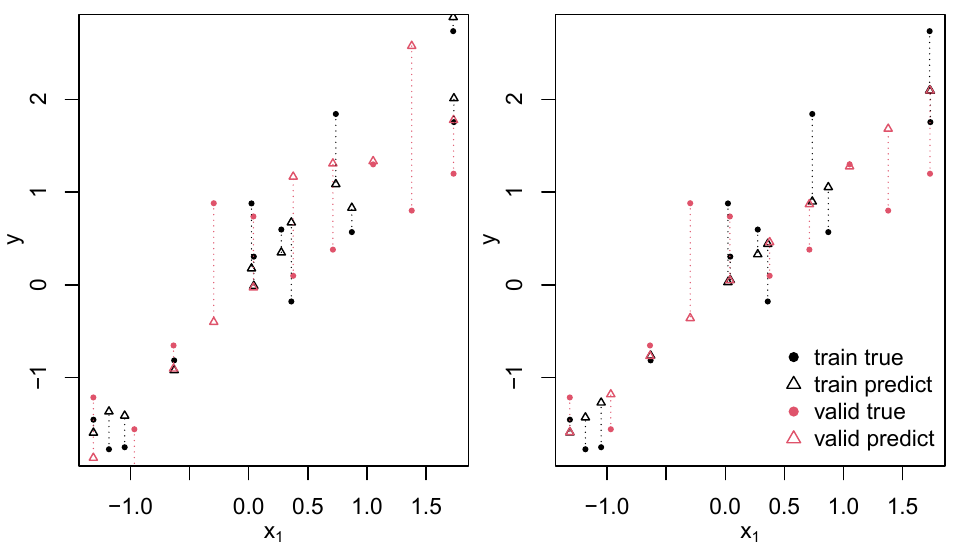
Toomet's demo uses twelve training rows, one real feature, and seven copies of it shaken by noise with standard deviation 0.005. The outcome is that feature plus noise of standard deviation 0.5. OLS training R-squared is 0.90, OLS validation R-squared is 0.09, and ridge validation R-squared is 0.54. Ridge training R-squared is 0.87, and forward selection's best one-feature model has validation R-squared 0.42, with a second feature flat beside it. The unconstrained fit spent its coefficients separating seven nearly identical columns. The penalty refuses that separation, and the validation fit survives.
Twelve rows, one signal copied seven times, no costs. Leave the 0.54 out of any Sharpe comparison. The old article "Can Machines Learn Weak Signals? Ridge > Zero > Lasso" is where ridge versus lasso is an empirical claim about weak signals. Use the 0.54 as a picture of what the penalty does to collinear copies.
At the desk, standardize, residualize, and print the sandwich
Center the features and scale them to unit variance before any lambda touches them. Leave the intercept out of W, or drop it after centering. Fit
beta-hat of lambda equals (X-transpose X plus lambda W) inverse times X-transpose y,
and when the feature count exceeds the number of days, use the n by n dual so you invert the small matrix. Pick lambda by a purged walk-forward, not by the in-sample residual sum of squares. The in-sample sum falls as lambda falls, and it will send you back to the singular OLS fit.
Read a controlled slope through Frisch-Waugh-Lovell. Residualize the controls out of the feature. Residualize the response too if the residual itself is an input to the next step, a sizing rule or a second regression. If you only residualize the feature, keep the coefficient and throw the residuals away. Multiply a homoskedastic standard error from that partial regression by the square root of (n minus l) over (n minus k minus l). Or skip that patch and print HC0, which already matches.
On a cross-section of assets, print HC3 when a few names dominate the hat diagonal, and at least HC0 otherwise. On an overlapping or otherwise serially correlated return, print Newey-West and set the lag to the overlap you built. The old article "Ridge Above 1h, XGBoost Below 5min" already tells you which model to point at a horizon above one hour. This is the estimator and the standard error you compute when that model is ridge.
The same diagonal load shows up when the matrix you invert is a covariance rather than X-transpose X. A singular 2 by 2 sample covariance with entries 0.04 and 0.02 off the diagonal, and 0.04 and 0.01 on it, has eigenvalues 0.05 and 0 and determinant 0. You cannot invert it for a minimum-variance weight. Shrink toward the average variance, here 0.025, with intensity 0.20:
$$ \hat{\Sigma} = (1-\delta)\, S + \delta \, v \, I = 0.8\, S + 0.005\, I = \begin{pmatrix} 0.037 & 0.016 \\ 0.016 & 0.013 \end{pmatrix}. $$
The eigenvalues move from 0 and 0.05 to 0.005 and 0.045. The condition number is 9, and the inverse exists. That spherical target is the covariance version of adding a multiple of the identity. Rahaman's section 6.2.2 prints the Ledoit-Wolf combination delta times F plus (1 minus delta) times S, with F the constant-correlation matrix whose off-diagonals are sigma-i times sigma-j times the average correlation. His introduction says that constant-correlation shrinkage is formally equivalent to ridge regularization of the sample covariance. The later section prints the convex combination and does not derive the equivalence. A constant-correlation F equals a multiple of the identity only in special cases. Use the formula in section 6.2.2 when you want his target, and use a multiple of the identity when you want the ridge load above. Do not treat the introduction's sentence as the derivation.
None of these notes contains a Sharpe ratio you should trade. Van Wieringen, Ding, and Toomet teach the linear estimator. Rahaman's review maps the quant toolkit and reports no tradable Sharpe. The old article "The Limits of Linear Models" is where a linear forecast fails even after the algebra is right. Fit the coefficient with the inverse that exists, print the standard error that matches the dependence you built, and then make the fit beat a purged out-of-sample test. The stack does not do that last part for you.
KEY POINTS
- Add lambda to the diagonal of X-transpose X before you invert. On van Wieringen's four-row design the smallest coefficient is 0.066 at lambda equal to 1 and 0.002 at lambda equal to 10.
- Keep eigenvalue over eigenvalue-plus-lambda of each direction. Eigenvalues 10 and 6 at lambda equal to 1 keep 0.91 and 0.86, the zero eigenvalue keeps nothing, and three columns spend 1.77 degrees of freedom.
- Residualize the controls out of the feature, then regress. The slope matches the multiple regression: 1.46 on the worked rows. Residualize the response too if you need the same residuals.
- Put each squared residual in the middle of the sandwich, and on an overlapping return add Bartlett-weighted lags. At 2,520 daily rows the review's rule of thumb floors that lag at 8, which still drops a 21-day overlap.
- Treat the twelve-row picture as a mechanism demo. OLS validation R-squared is 0.09 and ridge validation R-squared is 0.54, on seven noisy copies of one feature. Leave it out of the P&L.
References
- The Mathematics of Machine Learning, for Traders
- Can Machines Learn Weak Signals? Ridge > Zero > Lasso
- The Limits of Linear Models
- Ridge Above 1h, XGBoost Below 5min
- Lecture notes on ridge regression
- Linear Model and Extensions
- Lecture Notes for Machine Learning and Data Science Courses
- A Comprehensive Review of Statistical Methods in Quantitative Finance: From Classical Inference to Machine Learning Frontiers
A note on AI. The ideas, research, analysis, and conclusions in this article are my own. I use AI tools to help with editing and wordsmithing, because English is not my first language, and I am not shy about that. AI-generated ideas and AI-assisted writing are not the same thing: the first is empty slop from a generic prompt, the second is a tool for communicating years of real research more clearly. Judge the work by its substance, not by whether software helped polish the prose.