4.84 The Curl of Money: Decompose FX Into Currency Value and Arbitrage Loops

A ten-currency spot book, the USD, EUR, JPY, GBP, AUD, CAD, CHF, HKD, SGD, and SEK set in the old article "Graph Learning for FX: Interest-Rate-Parity Statarb Done Right," is a field of rates with one number on every pair. The quotes that follow are a constructed snapshot: EURUSD at 1.10, USDJPY at 150, EURJPY at 164. Walk one euro into dollars, those dollars into yen, and the yen back into euros, and you hold 165/164 euros, a cash gap of 1/164, or 0.61 percent, before any spread. That gap is a loop: one value per currency makes every closed path cancel, so the 0.61 percent has no home in the values. You forecast the change in the values, and you trade the loop only after a lagged-quote test leaves it standing and the gap clears the three spreads, the execution lag, and the weight a flat-holdings book will give you.

One value per currency soaks up every consistent rate

Hong and Klabjan write the quoted rate from currency i to currency j, the amount of j you receive for one unit of i, as a ratio of two currency values times a residual. In logs, the rate is the gap between the two log-values plus that residual. Before any of this they replace each pair by the geometric average of the two directions, so the log-rate from j back to i is the negative of the log-rate from i to j. The old article already ran their two-stage graph network on top of that book. The object underneath the network is the split.

Treat the log-value as a height assigned to the currency. The log-rate is the drop from one height to the other. Heights are free up to an additive constant, so the average height is pinned at zero. Hong and Klabjan's equations (8) and (9) are that fit, on a single snapshot.

$$ \log V_i - \log V_j = \log X_{ij}, \qquad \frac{1}{|C|} \sum_{i \in C} \log V_i = 0 $$

The first line asks every pair's log-rate to equal the height gap. On a book that contains a loop, no set of heights can hit every pair, so you solve the line in least squares and minimize the sum of squared misses. The second line removes the free additive constant. |C| is the number of currencies. Hong and Klabjan note that the rate rows alone have rank one less than |C|, which is why the average-height row is there. They treat the miss as Gaussian noise with mean zero, and under that assumption the least-squares heights are the maximum-likelihood values. A loop you can trade is a miss whose mean differs from zero. The projection onto heights is still the split you want. The zero-mean likelihood is the piece you drop when the residual is the position.

On a complete book, every pair quoted and the field antisymmetric, the least-squares height is the average log-rate out of that currency.

$$ v_i = \frac{1}{|C|} \sum_{j \neq i} \log X_{ij} $$

Each currency's log-value is the average of its log-rates against the others. The average of those log-values is zero by itself, because every log-rate enters once up and once down. On the snapshot, |C| is 3. The euro's log-value is (log 1.10 + log 164) / 3, which is 1.731726. The dollar's is (log 150 - log 1.10) / 3, which is 1.638442. The yen's is minus (log 164 + log 150) / 3, which is -3.370167. Euro minus dollar is 0.093284. The quoted log EURUSD is log(1.10) = 0.095310. The miss is 0.002026 in log points. The value-implied EURUSD is exp(0.093284), which is 1.0978, against the quote 1.1000. Exponentiate the log-values and the levels in the imaginary numeraire are about 5.650, 5.147, and 0.0344, with geometric mean 1.

That height gap is the gradient of the rate field. Hong and Klabjan do not use the word. Equations (8) and (9) are the gradient fit, and the miss they leave is the rest of the field.

A missing pair drops the average formula. You go back to the least squares and leave that row out. When they build the values they forward-fill a missing rate for up to seven days, and only for this fit. A seven-day fill is a stale height.

The loop is the part that sums around the triangle

The residual on a pair is the quoted log-rate minus the height gap.

$$ a_{ij} = \log X_{ij} - (v_i - v_j) $$

Walk the heights around a triangle and you are back at the start. The residuals remain. Their sum is the circulation, and it equals the sum of the quoted log-rates, because the heights contributed (v_i - v_j) + (v_j - v_k) + (v_k - v_i), which is zero. The circulation is the curl: the part of the field orthogonal to every height assignment. On a connected complete snapshot the gradient piece and this curl use up the whole field.

$$ C = a_{ij} + a_{jk} + a_{ki} = \log X_{ij} + \log X_{jk} + \log X_{ki}, \qquad \exp(C) - 1 $$

C is the log circulation. Exponentiate it and subtract 1 and you have the cash gap on one unit pushed around the cycle. On the snapshot the paying cycle is euro to dollar, dollar to yen, yen to euro. The product of the rates is 1.10 times 150 divided by 164, which is 165/164. The cash gap is 1/164, or 0.6098 percent, which is 60.98 basis points. The log circulation is log(165/164) = 0.006079. Exponentiate that and subtract 1 and you recover 1/164. On a three-currency book the three loop residuals are equal, each one third of the circulation, so each is 0.002026. Three times 0.002026 is 0.006078. The last 0.000001 is display rounding. In log-basis-points that residual is 20.26 on each leg, and the legs add to 60.79.

Look at the right-hand bar. It is the sum of the three legs, and it is the log of the cash gap.

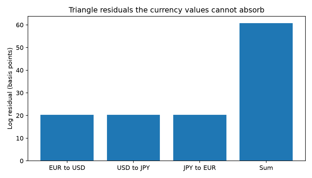
Hong and Klabjan's printed triangle line sets the rate from i to j equal to the rate from i to k times the rate from j to k. Under their own definition the middle factor would be the amount of k per unit of j, and the cycle they describe (i to k, then k to j, then j to i) wants the rate from k to j in that slot. The cash product that matches the definition is the rate from i to k, times the rate from k to j, times the rate from j to i, minus one. The printed subscript order on that line may be wrong. The numbers above follow the definition.

Fitting the heights again does not shrink C. The heights cancel on every closed path, so a real loop stays in the residual no matter how carefully you estimate V.

A lagged quote can fake the whole loop

A triangle stamped with one timestamp can be three quotes from three different milliseconds. The third leg is a late copy of the first two, the circulation is a stale print, and the partial correlation of the gap with that leg, given the lagged quote, is what kills it.

Runge and coauthors built the test on climate series. PCMCI, a parent screen followed by a momentary conditional independence test, is the version that still has power when the book is wide and the series are autocorrelated. The old article "Stop Using Pairwise Granger: PCMCI for Financial Causality" is that test in markets. The old article "Stop Using Pairwise Granger (causality upgrade)" is why you run it on the book rather than on the pair. The series you hand it here is the circulation.

Their linear version, partial correlation, regresses both series on the conditioning set and correlates the residuals. They do not print the one-conditioner reduction. With a single lagged quote q it is the usual formula.

$$ \rho(g, s \mid q) = \frac{\rho(g, s) - \rho(g, q)\,\rho(s, q)}{\sqrt{\big(1 - \rho(g, q)^{2}\big)\big(1 - \rho(s, q)^{2}\big)}} $$

The numerator removes the slice of the raw correlation that both series share with the lagged quote. The denominator rescales what remains. Work a stale quote in population, so sampling noise is out of the number. Let q, e, and u be independent with variance 1. Let the log-circulation be g = 0.8 q + e, and let the suspect leg be s = 0.6 q + u. The variance of g is 1.64, the variance of s is 1.36, and the covariance is 0.48. The raw correlation is 0.48 divided by the square root of the product 1.64 times 1.36, which is 0.3214. The correlation of g with q is 0.8 over the square root of 1.64, which is 0.6247. The correlation of s with q is 0.6 over the square root of 1.36, which is 0.5145. The product of those two is 0.3214, the numerator is zero, and the partial correlation is zero. The loop was the lagged quote.

A residual that shares an innovation with the leg survives the same arithmetic. Let g = 0.4 q + e and s = 0.4 q + 0.5 e + u, with the same independent unit-variance noise. The raw correlation is 0.516. After both series are regressed on q, the residual correlation is 0.5 divided by the square root of 1.25, which is 0.447. That is the partial correlation. The lag took a slice out of the raw 0.516 and left a dependence that is still there.

With a real parent set, the momentary conditional independence test is the same partial correlation with two conditioning collections in place of the single q: the parents of the circulation, and the parents of the driver, with the driver itself removed from the circulation's parents. Runge leaves same-bar links undirected, so the test does not arrow the three legs inside one snapshot. It tells you whether the gap still depends on a leg once the lagged quotes that could have manufactured it are conditioned out. A partial correlation of zero is a stale print. A partial correlation that holds is a candidate loop, and it still has to clear the costs below.

I am against sending the triangle on the snapshot that created it.

Directional FX is the change in those values

Between two snapshots the pair's log-change splits into the change in the height gap and the change in the residual.

$$ \Delta \log X_{ij} = \big(v_{i,t} - v_{i,t-1}\big) - \big(v_{j,t} - v_{j,t-1}\big) + \big(a_{ij,t} - a_{ij,t-1}\big) $$

The first two terms are the directional bet, which currency got taller in the imaginary numeraire. The last term is the change in the residual. A forecast of the pair is a forecast of both, added together. Move the snapshot to a second constructed print, EURUSD 1.12, USDJPY 148, EURJPY 166, and recompute the heights with the same average. The euro's log-value rises by 0.010047, the dollar's falls by 0.010481, and the yen's rises by 0.000434. Those three changes sum to zero, as they must if each day's heights do. The height-gap change on EURUSD is 0.010047 minus a dollar change of -0.010481, which is 0.020527. The quoted log-change is log(1.12) minus log(1.10), which is 0.018018. The residual change is 0.018018 minus 0.020527, which is -0.002509. Add 0.020527 to -0.002509 and you land on 0.018018. The pair's log-rally was a height gap of 0.020527, partly given back by a shrinking loop.

You forecast the height changes. The old article "Network Momentum as a Cross-Asset Factor" already turns a neighbor-weighted average of momentum features into a position. Feed it these log-value changes, for the currencies and for the other asset classes that article uses, and keep the residual change out of the feature. Pu, Roberts, Dong, and Zohren estimated that neighbor graph on 64 futures, from volatility-scaled returns and a normalized moving-average crossover. The propagation is theirs. The input is the height change.

The gap has to clear three spreads, then the lag, then the weight

The cash gap and the bill for crossing three spreads live in the same units, so you subtract.

$$ \Pi = \frac{X_{\mathrm{EU}}\, X_{\mathrm{UJ}}}{X_{\mathrm{EJ}}} - 1, \qquad S = \frac{0.0001}{X_{\mathrm{EU}}} + \frac{0.01}{X_{\mathrm{UJ}}} + \frac{0.01}{X_{\mathrm{EJ}}} $$

Π is the cash you keep on one unit pushed around the cycle, if every fill matches the snapshot. S is one pip on each leg as a fraction of the price: 0.0001 on EURUSD, and 0.01 on each yen pair. On the fat snapshot, Π is 1/164 = 0.006098. The three pips are 0.0001/1.10, 0.01/150, and 0.01/164, which are 0.91, 0.67, and 0.61 basis points. They sum to 2.19 basis points. The fat loop clears that bill with 58.8 basis points left. A one-yen miss on EURJPY is a teaching gap. A dealer snapshot is a few pips wide.

Scale the same identity. Leave EURUSD at 1.10 and USDJPY at 150, so the cross-implied EURJPY is 165, and print EURJPY at 164.98. The cash gap is 0.02/164.98, which is 1.21 basis points. The spread bill is still 2.19 basis points. The loop is behind on spreads alone.

The lag is that bill again if you budget one pip of move on each leg between the snapshot and the fill. Hong and Klabjan maximize the information ratio, expected gain over its standard deviation, because the rate at the observation differs from the rate at the execution. Another 2.19 basis points, and the 1.21 basis point triangle is a loss of 3.17 basis points: two spread-and-lag bills of 2.19, minus the 1.21 gap. The fat teaching triangle still clears a one-pip lag. A live triangle usually fails that budget.

The projection shows up as a weight. The trading book forces expected holdings to zero in every currency but the home currency, refuses both directions of one pair, and normalizes the positive weights so they sum to 1. The old article walks through that constraint set. The concentration they report is the number you need. The Herfindahl-Hirschman index is the sum of squared weights. On the USD book it prints at 31.60 for the linear program and 5.38 for the graph method, under a header that marks the table as percent, so those figures are 0.3160 and 0.0538. One over the index is the effective number of positions: 3.16 for the linear program, 18.59 for the graph method. The cash gap is earned on the slice of the book the projection leaves on that cycle.

The information ratio rose while the annual return fell

Look at the right-hand bar in the left panel. That is their graph neural network, marked GNN in the table, and its printed information ratio on the USD book.

The information ratio prints at 43.86 for the graph method and 27.21 for the linear program. The annual return prints at 4.80 against 6.19. The rest of the USD column is volatility 0.68 against 1.41. Across USD, EUR, and JPY the printed average changes are a Sortino ratio 45.51 percent higher, volatility 52.23 percent lower, and maximum drawdown 44.77 percent lower. Sortino here is expected gain over downside deviation. The average return change they print as -22.73 comes out to -22.76 if you average the three changes from the printed returns, so that cell may have been rounded before it was averaged. Return divided by volatility on those USD rows is 4.39 for the linear program and 7.06 for the graph method. The printed information ratios are 27.21 and 43.86. Annualizing the printed volatility by the square root of 252 lands at 27.65 and 44.47. The paper states neither a day count nor a return definition that would close that gap, and the source may be inconsistent. The printed ratios stay as printed.

The directional half of the split is already in the old article "Network Momentum as a Cross-Asset Factor." An FX sleeve fed by the full cross-asset graph has a Sharpe ratio of 0.66. The same sleeve fed by an FX-only graph has a Sharpe ratio of 0.16. That gap is the height-change sleeve. The circulation test above is the residual.

What you run before the open

Build the antisymmetric log-rates, fit the heights, and store the circulation of every triangle you can hit. Run the partial-correlation test of each circulation against its legs, conditional on the lagged quotes and on whatever else the parent screen kept. Drop every circulation whose partial correlation dies. Of what remains, keep a triangle only when the cash gap exceeds the three spreads plus the pip budget you assign to the lag. Size it at the projected weight. Forecast the height changes with the neighbor average, and keep the residual change out of that feature.

What they left out is the spread, the clock, and any driver missing from the file. Hong and Klabjan report those information ratios with no transaction costs, on daily bars, with unlimited borrowing at the government-bill rate in every currency, and with two-way arbitrage removed by the geometric average before the model sees a rate. Daily bars are the wrong clock for a triangle that lives for milliseconds. Pu, Roberts, Dong, and Zohren keep a positive Sharpe ratio on their futures book out to a 3 basis point cost and lose it by 5. That budget is a futures commission. A spot triangle pays three spreads, so the threshold you use is the pip sum above. Runge's test reads as causal only relative to the series you included. Leave the dollar funding basis out of the file and a circulation can look persistent because the basis is sitting in it. A link the test fails to find is the more trustworthy of the two answers.

Their write-up shows the rolling information ratio dropping hard in 2020, 2022, and 2024, and they tie those drops to shocks that were outside the training window. A loop rule fit on calm triangles pays those years back.

KEY POINTS

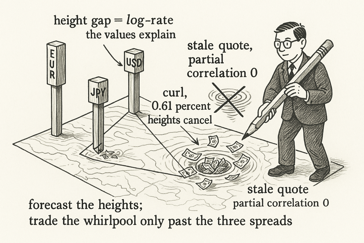
• Fit one log-value per currency as the average of its log-rates on a complete book. On the teaching snapshot the euro's log-value is 1.731726.
• Trade the circulation. The cash gap on EURUSD 1.10, USDJPY 150, and EURJPY 164 is 0.61 percent, and the heights contribute zero to it.
• Drop a loop whose partial correlation with the lagged quote is zero. The stale-quote case has partial correlation 0.
• Skip a curl inside the spreads. Three one-pip legs on the teaching quotes cost 2.19 basis points.
• Forecast the height changes, and judge the USD book by the printed information ratio of 43.86.

References

• Network Momentum as a Cross-Asset Factor
• Graph Learning for FX: Interest-Rate-Parity Statarb Done Right
• Stop Using Pairwise Granger: PCMCI for Financial Causality
• Stop Using Pairwise Granger (causality upgrade)
• Network Momentum across Asset Classes (Xingyue (Stacy) Pu, Stephen Roberts, Xiaowen Dong, and Stefan Zohren)
• Detecting and quantifying causal associations in large nonlinear time series datasets (Jakob Runge, Peer Nowack, Marlene Kretschmer, Seth Flaxman, and Dino Sejdinovic)
• Graph Learning for Foreign Exchange Rate Prediction and Statistical Arbitrage (Yoonsik Hong and Diego Klabjan)

A note on AI. The ideas, research, analysis, and conclusions in this article are my own. I use AI tools to help with editing and wordsmithing, because English is not my first language, and I am not shy about that. AI-generated ideas and AI-assisted writing are not the same thing: the first is empty slop from a generic prompt, the second is a tool for communicating years of real research more clearly. Judge the work by its substance, not by whether software helped polish the prose.