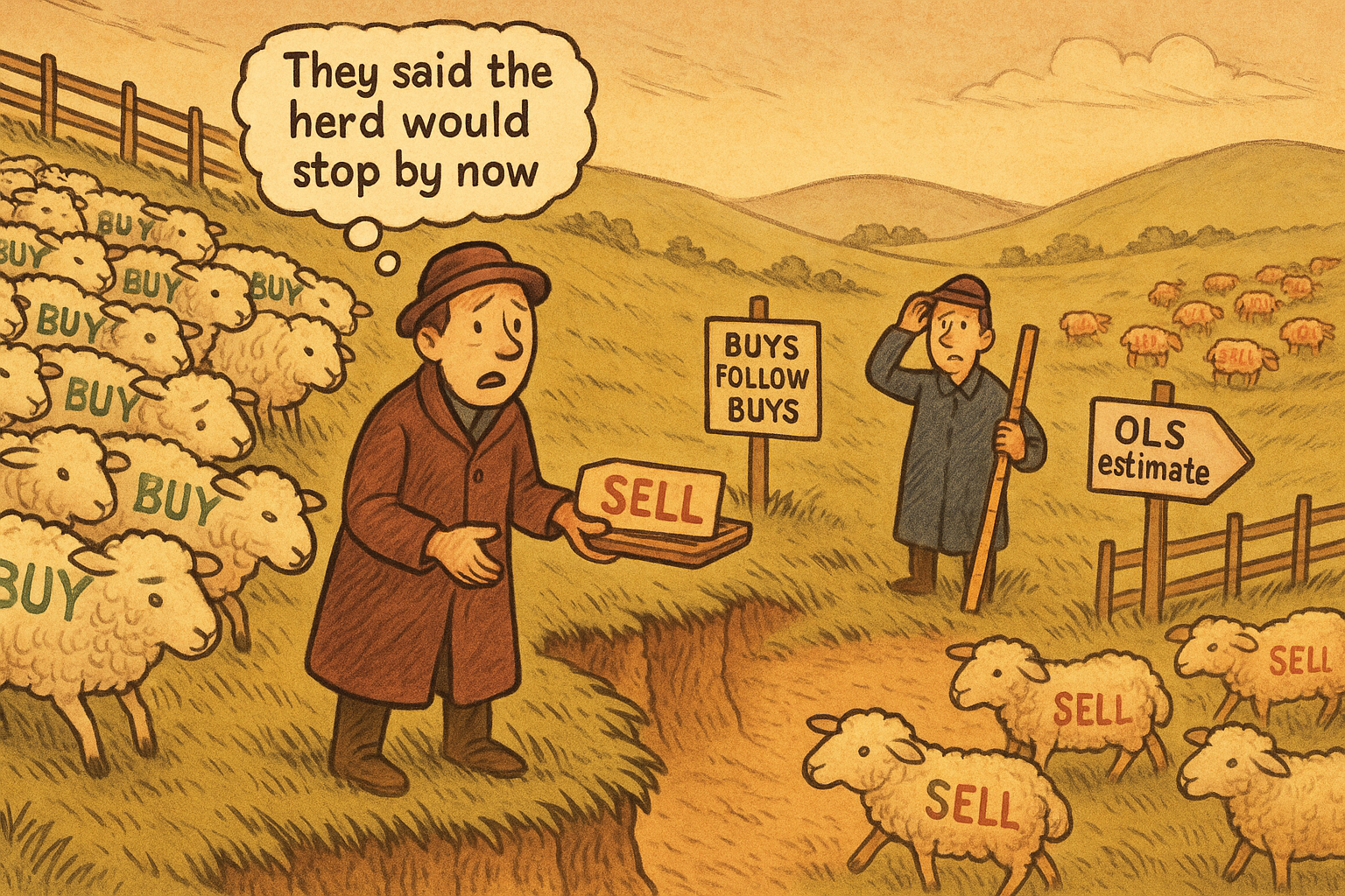
5. Microstructure Alpha July 2, 2026 5 min

5.30 Order-Flow Autocorrelation: Why Buys Follow Buys

Market orders are autocorrelated, roughly AR(1): buys follow buys in clustered spikes. Don't post offers into a buy run. And beware, OLS underestimates phi, so your model clears you to requote half a run too early.

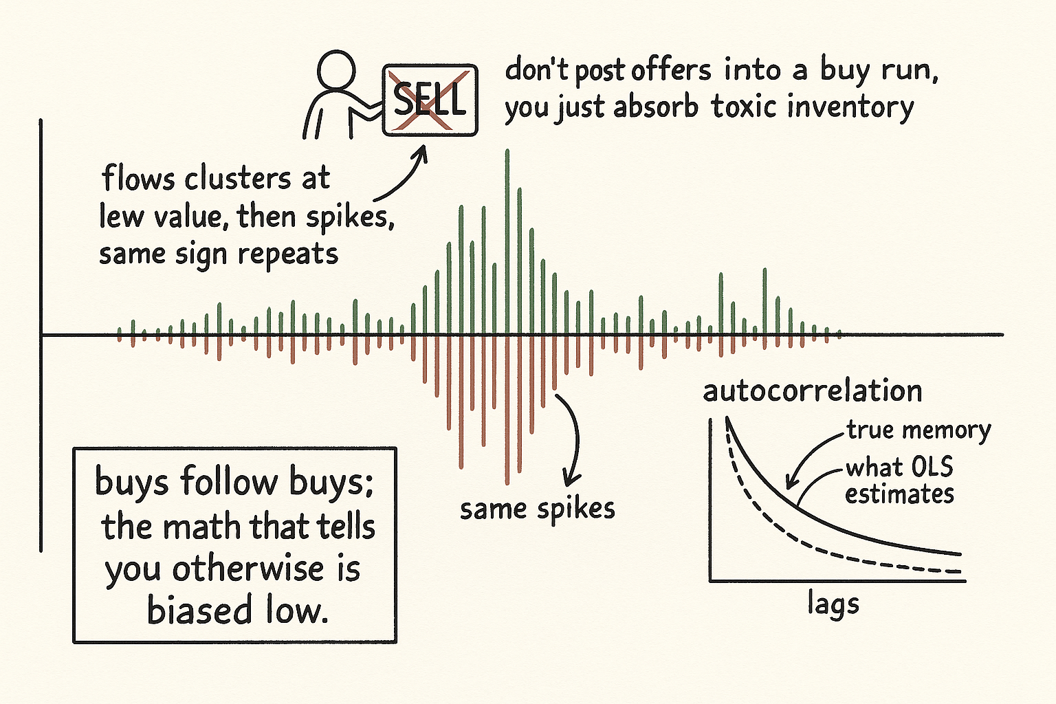
Sign every market order, plus for a taker buy, minus for a taker sell, and plot the series. You do not get random noise around zero. You get long stretches sitting near zero punctuated by sudden clusters of same-signed prints: a run of buys, then quiet, then a run of sells. Market order flow is autocorrelated, and the cleanest model for it is an AR(1) process, the same first-order autoregression that shows up everywhere a value depends mostly on its own immediate past.

The old article "Using Trade Flow to Predict Short-Term Price Movement" leaned on this fact without dwelling on it: trade flow predicts because market orders are roughly AR(1), so net signed flow over a window carries forward. This article is about why that is true, what the AR(1) structure actually implies, and the one trap that makes you systematically underestimate how long a run will last.

Why the flow clusters

The mechanics are not mysterious. A large order rarely executes in one print. A fund unwinding size slices it into children, so one parent buy becomes twenty taker buys in a row. Momentum chasers pile onto a move that is already happening, adding buys on top of buys. And the makers absorbing all of it react: when a maker gets lifted and goes short inventory, the old article "Order Book Imbalance: The First Microstructure Feature to Test" described how a thinned ask becomes the path of least resistance, so the next taker finds it even easier to buy. Each buy makes the following buy slightly more likely. That feedback is the autocorrelation.

The shape is distinctive: the flow clusters at a low value most of the time, then spikes. It is not a gentle sine wave of buying and selling. It is long quiet flat with occasional violent same-signed bursts, which matters because the bursts are where the price moves and where your inventory gets dangerous.

The AR(1) model and what it says

Write signed flow as a value that is mostly a fraction of its previous value plus a fresh shock.

$$ m_t = \phi \, m_{t-1} + \varepsilon_t, \qquad \varepsilon_t \sim N(0, \sigma^2), \qquad 0 < \phi < 1 $$

Read it as: this instant's flow equals phi times last instant's flow plus random noise. The phi is the memory coefficient. At phi near zero the flow is memoryless and yesterday tells you nothing; at phi near one the flow has long memory and a buy run takes a long time to die. The autocorrelation at lag k is phi to the power k, so a phi of 0.8 means flow one step ahead is still 80 percent correlated, two steps 64 percent, and the influence decays geometrically. For order flow phi is positive and often high at the sub-second scale, which is the formal statement of "buys follow buys."

The trap: OLS underestimates the memory

Here is the part that costs people money, and it is subtle. When you estimate phi by regressing the flow on its own lag with ordinary least squares, the estimate is biased low. The bias is structural, not a sample-size accident.

The reason is that in an autocorrelated series the regressor and the error term are entangled. Both m_t and m_{t-1} contain the same past shocks, epsilon at t-1, t-2, and so on, so the numerator and denominator of the OLS slope estimate share error terms. That shared dependence drags the estimated slope below the true one. In the positive-autocorrelation case the bias is negative, so your fitted phi comes out smaller than reality.

The consequence is direct and dangerous for a maker. Your model thinks there is structurally less memory in the flow than there really is. It expects a buy run to decay faster than it does, so it expects the pressure to fade, the price to settle, and your short inventory to become safe sooner than it will. You lean back into quoting offers too early, get filled again into the run that has not actually finished, and your inventory keeps climbing. The model underestimates both how long the run lasts and how far it can push, because the same bias that shrinks phi also makes the model underestimate the variance of the move.

The practical rule

The actionable takeaway needs no estimation at all: when you see a cluster of buy taker orders coming through, do not post sell limits into it. The resource says it plainly, and it is the entire trade. Selling into a buy-taker run hands those takers exactly the liquidity they want and leaves you holding the inventory while the run keeps going against you, the worst kind of fill, the one the old article on not getting filled warns is where nearly all of a maker's losses come from.

Concretely, this is a skew. When signed flow over your window is strongly positive, you skew your quotes up: pull your offer back or widen it so you are less likely to sell into the buying, and lean your bid in if you want to participate on the side the flow favors. This is the inventory-and-flow skew, now driven by the recognition that the flow is autocorrelated, so a positive reading is not a one-off, it is the start of a likely run.

A worked number

Suppose your true flow phi is 0.85 but OLS hands you 0.70. You see a buy run with current pressure at some level and you want to know how long until it decays to a tenth of its strength. With the fitted 0.70, the run decays as 0.70 to the power k, hitting one-tenth at about k = 6.5 steps, so your model says the pressure is gone in roughly 7 ticks and clears you to quote offers again. With the true 0.85, decay is 0.85 to the power k, reaching one-tenth at about k = 14 steps. The run lasts more than twice as long as your model believes. Quote offers at tick 7 and you are selling into seven more ticks of buying you did not price for. The biased phi did not look dangerous; it just quietly told you the all-clear half a run too early.

Visualizing the clustered flow

KEY POINTS

Signed market-order flow is autocorrelated and well modeled as an AR(1) process: this instant's flow is mostly a fraction phi of the last instant's flow plus a shock, so buys follow buys and sells follow sells.
The flow clusters at a low value with sudden same-signed spikes, not a smooth oscillation. The spikes are where price moves and where inventory gets dangerous.
Phi is the memory: autocorrelation at lag k is phi to the k. At the sub-second scale phi is positive and often high, the formal version of "buys follow buys."
OLS estimates of phi are biased low because the regressor and error share past shocks. Your model then thinks runs decay faster than they do and clears you to requote too early.
The practical rule needs no estimation: do not post sell limits into a cluster of buy takers. Selling into a run hands takers liquidity and leaves you holding inventory while price runs against you.
Act on it as a skew: when windowed signed flow is strongly positive, pull or widen your offer and lean your bid, treating the reading as the start of a likely run rather than a one-off.