9.27 CVaR Sizing: One Tool, Two Markets
The CVaR-constrained portfolio QP that sizes Polymarket election arbs is the same machine that sizes a futures book. Different loss shapes, one tail metric, one fix for the correlation that spikes in a crisis.
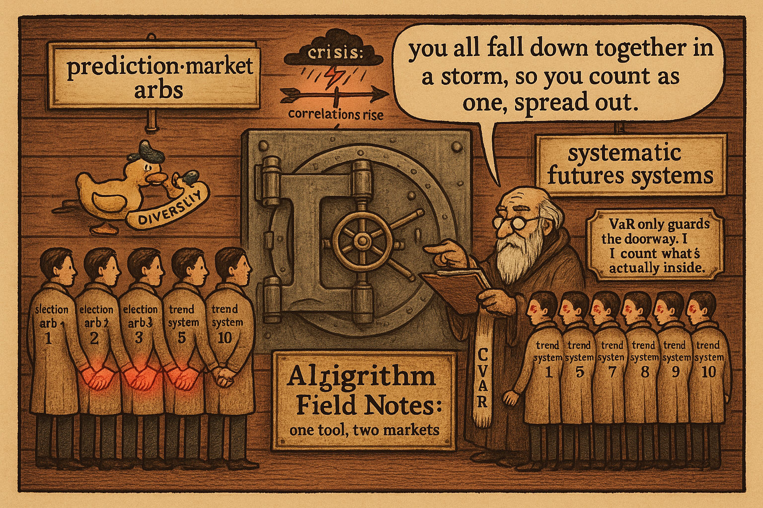
Five Polymarket election arbs that each look independent all lose together when one national result surprises. Ten trend-following futures systems that each look independent all bleed together in the same choppy regime. Different markets, different instruments, identical failure: a book of individually-good positions that is secretly one bet, and a risk model that priced them as many. The tool that stops both is the same conditional-value-at-risk constraint inside the same quadratic program, and once you see it work on election arbs you already know how to run a systematic futures book.
The article "Kelly Isn't Enough" built the CVaR-constrained portfolio QP for prediction-market arbitrage. This is that machine pointed at the other pillar. The prediction-market half of it is the correlated blowup of arbitrage legs; the systematic half is what the old article "Smooth Equity Curves Are Built, Not Found" called the correlation that rises in a crisis exactly when you need it to stay low. Same math.
The number VaR hides, in both markets
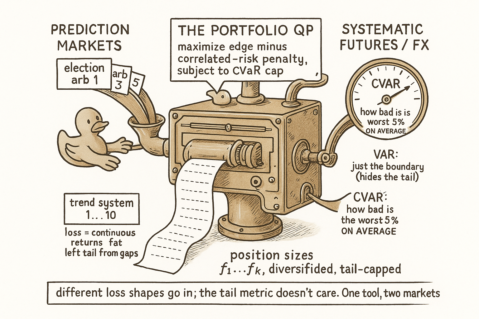
Value at Risk answers where the bad region starts and says nothing about what is inside it. Conditional Value at Risk answers the question that empties accounts: once you are past the boundary, how bad is it on average.
$$ \mathrm{CVaR}_\alpha = \mathbb{E}\big[\, \text{Loss} \;\big|\; \text{Loss} > \mathrm{VaR}_\alpha \,\big] $$
CVaR is the expected loss conditional on being past the VaR line. Sort 100 trades worst to best; say the worst five lose 80, 60, 45, 30, and 20 dollars. VaR at 95 percent is 20, the boundary. CVaR at 95 percent is the average of the five.
$$ \mathrm{VaR}_{95\%} = \$20, \qquad \mathrm{CVaR}_{95\%} = \frac{80 + 60 + 45 + 30 + 20}{5} = \$47 $$
VaR reports 20 and stops. CVaR reports 47, and the gap is the whole point: a strategy with a VaR of 20 and a CVaR of 200 has a fat tail VaR completely conceals. The old article "Fat Tails: Why Gaussian Thinking Breaks Trading Systems" made the systematic version of this argument, that a normal-distribution risk model sizes you for an ordinary day and an ordinary day is not when you blow up. CVaR is the answer in both places because it is defined on the tail itself, not on a Gaussian approximation of it.
The loss distributions differ; the tail metric does not
The two markets have different-shaped losses, and this is where people wrongly assume they need different tools. A prediction-market arbitrage loss is discrete, three branches, and the middle branch is the killer.
$$ \text{Loss} = \begin{cases} -(\Pi^* - \Delta) & \text{full execution (the intended profit)}\\ -(\text{partial cost} - \text{recovery}) & \text{partial execution (one leg stranded)}\\ 0 & \text{no execution} \end{cases} $$
Full execution pays the guaranteed profit, no execution costs only opportunity, and partial execution is where a hedged arb becomes a naked directional bet because one leg filled and the other did not. A systematic futures or FX strategy has no branches; its loss is a continuous return with a left tail fattened by gaps, regime shifts, and volatility clustering. Two completely different distributions. CVaR does not care. It reads the worst alpha percent of whatever distribution you hand it and reports the average loss there, so the same constraint bounds the partial-execution disaster on Polymarket and the gap-risk tail on a bund future without changing form.
One allocation, both books: the portfolio QP
Sizing positions one at a time misses the co-movement that does the damage. Allocate across the whole book at once.
$$ \max_{f_1, \ldots, f_k}\; \sum_i f_i e_i - \tfrac{1}{2}\, \mathbf{f}^\top \Sigma\, \mathbf{f} \quad \text{s.t.} \quad \sum_i f_i \le F_{\max},\;\; 0 \le f_i \le f_i^{\max},\;\; \mathrm{CVaR} \le C_{\max} $$
The first sum is total expected profit, each fraction times its edge. The covariance term with sigma is a penalty for correlated risk: when two positions tend to lose together, sigma grows and the optimizer holds less of both, forcing diversification the trader would not do by eye. The constraints cap total capital, cap each position, and cap the portfolio tail. This is a quadratic program, a squared objective with linear constraints, and CVXPY or OSQP or Gurobi solve hundreds of positions in milliseconds.
Read the covariance term through the systematic lens and it is the same object the old article "Why Portfolio Construction Is Part of the Signal" insisted on: how you weight and net correlated positions changes what the strategy predicts, so ten correlated energy futures equal-weighted are one bet stacked ten times, and the QP's sigma penalty is what stops you from stacking. The old article "The Difference Between Signal Quality and Portfolio Quality" split those into two dimensions; the QP is the construction dimension made explicit, the part that decides how much of a good signal you actually keep.
Where the correlation actually hides
The QP is only as honest as the sigma you feed it, and plain correlation lies in exactly the moments that matter. Five election arbs can show a linear correlation around 0.75 in calm conditions and a tail dependence near 0.90 when a national shock hits, so the joint extreme loss runs many times what the correlation predicts. The article "Correlation Lies; Tail Dependence Tells the Truth" is where the prediction-market pillar swaps the covariance matrix for a Student-t copula that captures joint tails. The systematic pillar reached the same wall from the other side: the old article "Smooth Equity Curves Are Built, Not Found" ends on the warning that correlations rise in crises, so the diversification that smooths your equity curve in normal times fails precisely when the crisis arrives. Two pillars, one defect in linear correlation, one fix, model the tail dependence and let CVaR bound the joint loss rather than the marginal one.
The systematic reader has one more familiar friend here. The old article "Average Drawdown vs Extreme Drawdown" separated the comfortable typical dip from the survival-question extreme, and used Monte Carlo permutation to build a distribution instead of trusting one realized max. That is the same move as simulating the loss distribution to estimate CVaR: you refuse to size off a single sample and you plan around the tail of the distribution, not its middle.
The through-line
CVaR does not raise your edge in either market. It stops the fat tail VaR cannot see and, wrapped in the QP with a covariance penalty, it stops the correlated blowup you did not price. On Polymarket that blowup is partial-execution losses correlating across arbs in a bad block. On a futures book it is ten systems that share a regime dependence and draw down as one. The article "Match Your Edge to Your Resources" argued that once the math is done the job is staying alive to collect the edge, and the CVaR-constrained QP is the single piece of machinery that does that job identically across both pillars.
KEY POINTS
- CVaR is the expected loss in the worst alpha percent of outcomes, not the boundary VaR reports. In the worked example VaR is 20 dollars and CVaR is 47; a VaR of 20 with a CVaR of 200 has a fat tail VaR hides. Constrain CVaR in both markets.
- Prediction-market arbitrage losses are three-branch and discrete, with partial execution the dangerous branch. Systematic-strategy losses are continuous with a gap-fattened left tail. CVaR is defined on the tail of whatever distribution you feed it, so the same constraint bounds both.
- The portfolio QP maximizes edge minus a covariance penalty subject to caps on total capital, per-position size, and portfolio CVaR. The covariance term forces diversification, and QP solvers handle hundreds of positions in milliseconds. It is the same machine for election arbs and a futures book.
- The covariance penalty is the systematic pillar's "portfolio construction is part of the signal" made explicit: ten correlated positions equal-weighted are one bet stacked ten times, and sigma is what stops the stacking.
- Plain correlation understates joint tails in both markets: election arbs show correlation near 0.75 but tail dependence near 0.90 under a shock, and systematic books see correlations rise in a crisis. Model the tail dependence and let CVaR bound the joint loss.
- CVaR raises no edge. It stops the fat tail VaR conceals and the correlated blowup a per-trade sizer never prices, identically across prediction markets and systematic trading.