4.75 Commodity Currencies: Predictable Only Where They're Thin

A one-standard-deviation rise in a country's commodity export prices predicts a 0.39% appreciation of its currency against the dollar over the next month. Jeanneret and Sokolovski find that slope in eight commodity-exposed currencies from January 1985 to April 2020, and the Australian dollar and the Canadian dollar contribute almost none of it. The forecast sits in the thinner names. In the Brazilian real, leveraged funds move the futures position with last month's export prices, while the Australian dollar's funds move it in the same month. I am against booking the 0.39% as payment for risk: export prices rise in months when the VIX is lower.

A commodity currency is the beta that survives the dollar

Export share is a bad screen. Colombia ships 68% of its exports as commodities and its currency beta on those prices is 0.18 with a t-stat of 0.73. Mexico ships 18% and gets 42% of government revenue from commodities; its beta is 0.60 with a t-stat of 2.48. Australia runs the other way on the fiscal side, 67% of exports and 2% of government revenue, with a beta of 0.52. The screen is the regression beta, after the dollar.

$$ \Delta s_{i,t} = \alpha_i + \beta_i \, \Delta CP_{i,t} + \gamma_i \, DOL_t + \varepsilon_{i,t} $$

The left side is the monthly percent change in dollars per unit of currency i, so a positive number is an appreciation. The commodity term is the standardized log change in that country's export-price index if it is a net exporter, and in its import-price index if it is a net importer. The dollar factor is the average percent change, that month, of the sample's currencies against the dollar. The beta is the percent appreciation that lines up with a one-standard-deviation commodity move once that average dollar move is held fixed. Jeanneret and Sokolovski standardize the commodity index, so a beta of 1 is a 1% currency move per one-standard-deviation commodity month.

Brazil, on 193 months, prints a constant of -0.18, a commodity beta of 0.87, and a dollar loading of 1.19. A month with a one-standard-deviation rise in Brazilian export prices and a 1% rise in the dollar factor has a fitted appreciation of -0.18 + 0.87 + 1.19, which is 1.88%. Colombia, on the same length of sample, has a commodity beta of 0.18 and a dollar loading of 1.22. The same two shocks fit -0.04 + 0.18 + 1.22, which is 1.36%, and 1.22 points of that is the dollar. Drop the dollar factor and 22 of the 40 currencies look commodity-exposed, including importers whose whole correlation is the dollar price of commodities. With the dollar in the regression, eight exporters clear a positive beta at 10%: Australia 0.52, Brazil 0.87, Canada 0.40, Mexico 0.60, New Zealand 0.30, Norway 0.28, Peru 0.24, Russia 1.41. Five importers clear a negative beta: the euro -0.30, Japan -0.46, Switzerland -0.26, the Philippines -0.23, Thailand -0.27. South Africa's beta of 0.32 stops at a t-stat of 1.61, short of that 10% line. The ruble is the one currency that loads on both baskets; in the joint regression the export loading is 2.01 and the import loading is -0.86.

One standard deviation of export prices leaves 0.39 percent for next month

The beta above is the same-month move. The forecast is last month's export-price change against this month's currency change, on the eight exporters, with a separate intercept for each currency.

$$ \frac{1}{k}\Delta s_{i,t+k} = \alpha_{i,k} + \delta_k \, \Delta CEP_{i,t} + \theta_k x_t + u_{i,t+k} $$

For a one-month horizon, k is 1 and the left side is next month's percent appreciation. The export-price change is standardized, so the slope is the percent appreciation that follows a one-standard-deviation rise. The controls in x are the interest differential implied by the one-month forward, the real exchange rate, last month's currency change, the dollar factor, the change in average FX volatility, the change in the TED spread, the change in the VIX, and an NBER recession indicator. Standard errors are Driscoll-Kraay with a Newey-West kernel. With every control included, the one-month slope is 0.390 with a standard error of 0.112. Divide those and the t-stat is 3.48, which is the t-stat they print.

A one-standard-deviation month therefore lines up with 0.390% of appreciation over the next month. Scale the month by twelve: 12 times 0.390 is 4.68%, which the paper rounds to 4.7%. That 4.68% is twelve repetitions of the one-sigma month. The paper does not report a strategy Sharpe on this regression. The panel R-squared on the full control set is 2.09%. Across the nine columns of their control table the slope stays between 0.379 and 0.407. The interest differential, lagged FX, the dollar, volatility, the TED, the VIX, and the recession dummy do not move it. The real exchange rate is the other coefficient that clears 5%, at -0.020 with a standard error of 0.008, and the paper does not state the units of that real rate, so the -0.020 stays a control. Replacing the spot change with an excess return, spot plus the interest differential, leaves the export-price slope essentially unchanged.

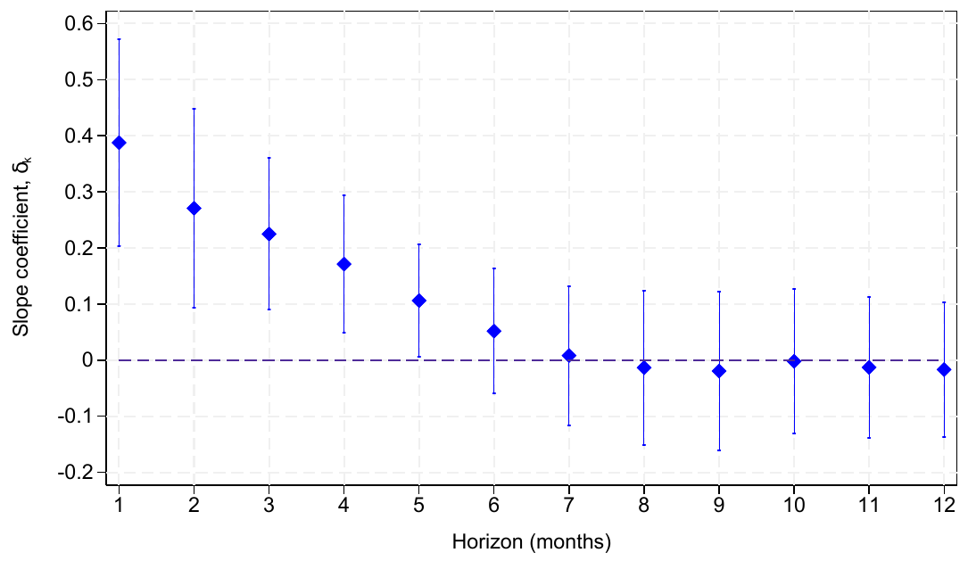
The left side divides by k, so at a six-month horizon the slope is the average monthly appreciation over those six months. The six-month total is k times that average. If the entire 0.39% arrived in month one and later months added nothing, the six-month slope would be 0.390 divided by 6, which is 0.065. The figure below is that slope at each horizon. The diamond at one month is the 0.39. The interval covers zero from about month five, which is the paper's statement that the forecast is negligible after five months.

Split the eight exporters by BIS daily turnover, averaged from the triennial surveys of 2004 to 2019. The six below Australia and Canada print a slope of 0.523 with a standard error of 0.126, a t-stat of 4.15, and an R-squared of 2.97%. Twelve times 0.523 is 6.276% in a one-sigma month. Australia and Canada together print 0.145 with a standard error of 0.120, a t-stat of 1.21, and an R-squared of 0.42%. The importer panel is the same pattern at a weaker significance. All five importers together print -0.052. Drop the euro, the yen, and the Swiss franc, and the Philippine peso and the Thai baht print -0.210, significant at 10%. A one-standard-deviation rise in their import prices lines up with a 0.21% depreciation next month, 2.52% scaled by twelve. The three liquid importers print 0.013.

Country export prices survive a world commodity index. Adding the CRB change cuts the panel slope from 0.388 to 0.284, and it stays significant at 5%. Adding the GSCI cuts it to 0.320. New Zealand, whose basket is dairy and meat, has its own slope of 0.530, which falls to 0.431 with the CRB and to 0.458 with the GSCI. The country basket is the regressor.

The leftover slope is the price weight that did not use the news

Their appendix writes a three-date model in which one group of traders updates on the public commodity news and another group treats the exchange rate as a random walk. The price is a weighted average of those two valuations, so part of the news is missing from this month's rate and shows up in next month's change. The regression slope on the news, the object that corresponds to the 0.39, is the product of two weights.

$$ \beta_1 = \eta \, (1 - \omega_I), \qquad \eta = \frac{\sigma^2}{\sigma^2 + \sigma_\epsilon^2} $$

The signal weight, eta, is the share of the news variance that is the fundamental, fundamental variance over fundamental variance plus noise variance. The informed weight, omega-I, is the share of this month's exchange rate set by traders who use the news. When that share is 1, the slope is zero: the news is already in the price. When that share is lower, the slope rises toward the signal weight. The appendix first writes the next-month change as (1 minus omega-I times eta) times the news. That reading treats the signal's own noise as uncorrelated with the news, and the residual in that line contains the signal's noise, which is correlated with the news. The covariance algebra two pages later, their derivation A.8.2, produces eta times (1 minus omega-I). That is the slope a regression recovers. With a signal weight of 0.5 and an informed weight of 0.2, the two expressions give 0.90 and 0.40. I use 0.40.

The two estimated slopes are a sketch. The paper does not report these weights. Force both groups to share a signal weight, and the thick-currency slope of 0.145 and the thin-currency slope of 0.523 match a signal weight of 0.725, an informed weight of 0.800 in Australia and Canada, and an informed weight of 0.279 in the other six. Check: 0.725 times (1 minus 0.800) is 0.725 times 0.200, which is 0.145. And 0.725 times (1 minus 0.279) is 0.725 times 0.721, which is 0.5227, against the estimated 0.523. Any other pair of weights with the same products fits the same two numbers. The model is not identified off this pair. The sketch only shows the comparative static: an informed weight of 0.80 in the thick book and 0.28 in the thin book lines up with the two slopes when the signal weight is held fixed.

The same model says the slope should be larger when traders are less willing to take the other side. Demand for currency i at the news date is the gap between that trader's expected terminal rate and the current rate, divided by the variance of the terminal rate. Risk aversion is set to 1 in the appendix, so the position is in units of the log exchange rate over its variance.

$$ x_{i,1} = \frac{E_{i,1}[s_2] - s_1}{V_{i,1}[s_2]} $$

A gap of 0.01 with a variance of 0.01 is a position of 1. The same gap with a variance of 0.04 is a position of 0.25. Four times the uncertainty, a quarter of the position, and more of the news left for next month. The empirical version of that split is a dummy for lagged FX volatility in the top quintile of the eight exporters. Outside that quintile the export-price slope is 0.209 with a standard error of 0.141. Inside it, the slope is 0.209 plus an interaction of 0.466, which is 0.675. The interaction's t-stat is 0.466 divided by 0.206, which is 2.26. The base slope's t-stat is 1.48. Twelve times 0.675 is 8.10% in a one-sigma month during the stressed fifth of the sample, against 2.51% in the other months. They publish no Sharpe ratio on this split.

Leveraged funds add the position in the following month

The lagged position shows up in the CFTC's leveraged-funds category, the accounts with a reason to read a public oil price. The reports run from June 2006 to April 2020 and cover six of the eight exporters. The regression is the standardized monthly change in their net futures position on the standardized export-price change, with a dummy for the currencies whose out-of-sample R-squared is insignificant.

$$ \Delta Position_{i,t} = b_1 \, \Delta CEP_{i,t} + b_2 \, (\Delta CEP_{i,t} \times Efficient_i) + \alpha_i + \varepsilon_{i,t} $$

The dummy is 1 for the currencies that do not beat a random walk out of sample. On a one-standard-deviation export-price month, the position change in an inefficient currency is b1, which is 0.015 with a standard error of 0.047. In an efficient currency it is 0.015 plus 0.165, which is 0.180. The interaction's t-stat is 0.165 divided by 0.052, which is 3.17. Same-month positioning shows up where the return forecast does not.

The lag goes the other way, and it scales with futures turnover. Average daily volume over open interest, from CME reports, is 0.84 in the Australian dollar, 0.63 in Canada, 0.67 in New Zealand, 0.37 in Mexico, 0.12 in Brazil, and 0.05 in Russia. The lagged regression on the panel is a slope on last month's export-price change plus that slope times the turnover ratio.

$$ \Delta Position_{i,t} = 0.136 \, \Delta CEP_{i,t-1} - 0.195 \, \left(\Delta CEP_{i,t-1} \times \frac{ADV_i}{OI_i}\right) + \alpha_i + e_{i,t} $$

Both coefficients are from their column that interacts the lag with the turnover ratio: 0.136 with a standard error of 0.068, and -0.195 with a standard error of 0.109. At Brazil's ratio of 0.12 the fitted lag is 0.136 minus 0.195 times 0.12, which is 0.113. At Australia's ratio of 0.84 it is 0.136 minus 0.195 times 0.84, which is -0.028. The lag crosses zero at 0.136 divided by 0.195, a turnover ratio of 0.70. The single-currency case study matches the sign of that panel. The Australian dollar's same-month position slope is 0.122, significant at 5%, with an R-squared of 2.91%, and the lag is -0.049 with an R-squared of 0.47%. The real's same-month slope is -0.105 with an R-squared of 0.97%, and the lag is 0.220, significant at 5%, with an R-squared of 3.88%.

How many days that lag takes is a participation limit. The target position is a fraction p of open interest. The cap is a fraction alpha of average daily volume, so the order does not become the whole tape.

$$ T = \frac{p \cdot OI}{\alpha \cdot ADV} = \frac{p}{\alpha \cdot (ADV / OI)} $$

They set p to 0.10 and alpha to 0.05, which collapses the expression to 2 divided by the turnover ratio. On the printed ratios that is 2 divided by 0.84, which is 2.38 days in the Australian dollar, and 2 divided by 0.12, which is 16.67 days in the real. Russia's ratio of 0.05 gives 40.0 days. Table 5 prints 2.6 days and 25.6 days in the same cells as 0.84 and 0.12. Those day counts disagree with 2 divided by the ratios beside them, and 25.6 divided by 2.6 is 9.85 while 0.84 divided by 0.12 is 7.00, so the printed days are out of proportion with the inverse of the printed ratios. The prose says "less than 3" and "roughly 26," which matches the table's day counts. The formula on the ratios matches 2.38 and 16.67. I keep both. Either pair says the real takes several times longer than the Aussie. The source's arithmetic on the pair of numbers does not close, and the table may be using a volume series that is not the ratio it prints.

New Zealand breaks a clean ranking by futures turnover. Its ratio is 0.67, next to Canada's 0.63, and the interaction above puts its lagged position response at 0.136 minus 0.195 times 0.67, which is 0.005, essentially zero. Its currency still has an out-of-sample R-squared of 1.03. The futures-turnover channel is a Brazil-versus-Australia fact. It does not sort the New Zealand dollar from the Canadian dollar. Dollar turnover does: 82 billion a day against 212 billion.

A higher VIX is the wrong state for this forecast

A risk premium is larger in the riskier state. Here the predicted appreciation is positive after export prices rise, and the months when export prices rise are months when risk measures fall. The regression is contemporaneous, on the equal-weighted average of the eight exporters' standardized export-price changes.

$$ VIX_t = a + b \, \Delta \overline{CEP}_t + e_t $$

The slope b is -2.03 with a standard error of 0.69, and the constant is 20.15. A one-standard-deviation commodity month lines up with a VIX of 20.15 minus 2.03, which is 18.12, against a sample mean of 20.15. The same commodity month lowers the Bekaert risk-aversion index by 0.19, the Jurado macro-uncertainty index by 0.57, and the excess bond premium by 0.13. Local equity indexes in Brazil, Canada, Mexico, Norway, Russia, and Peru rise with the country's own export prices in the same month. Australia and New Zealand are positive and insignificant. A positive currency forecast in a state with a lower VIX, lower risk aversion, and higher local equities is the wrong sign for compensation. Risk-premium forecasts in equities also tend to strengthen as the horizon lengthens. This slope is gone by month five.

The out-of-sample gain sits under 100 billion of daily turnover

Look at the top panel. Red diamonds are the currencies whose commodity forecast beats a random walk with drift at 5%. Every one of them has average daily turnover below 100 billion dollars. The line falls as turnover rises: slope -0.011, cross-sectional R-squared 54%.

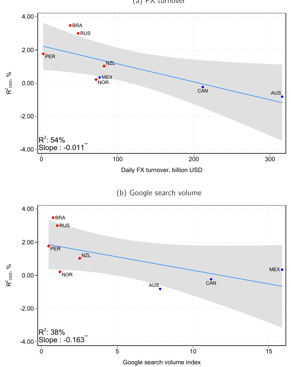
Brazil's out-of-sample R-squared is 3.48. Australia's is -0.81. With the six thinner commodity currencies removed, the carry slope is 0.16 and insignificant.

The rest of the grid: Russia 3.00, Peru 1.77, New Zealand 1.03, Norway 0.22, Mexico 0.35, Canada -0.23; the full carry slope is 0.312, and 12 times 0.312 is 3.74%, its out-of-sample R-squared is 0.87, and that R-squared is -0.20 with the six thin names removed, while the stripped carry still earns 7.90% a year against 8.61% for the full book. The out-of-sample statistic is Campbell and Thompson's: one minus the ratio of mean squared errors, commodity forecast over a random walk with drift, on an expanding window that starts with 24 months. They set the slope to zero in any window where its sign disagrees with the currency's commodity beta. Brazil's 3.48 means the commodity forecast's squared errors are 96.52% of the random walk's, because 1 minus 0.0348 is 0.9652. Australia's -0.81 means the commodity forecast is worse than the expanding mean. Canada's -0.23 is also a loss to the random walk; the table stars it at 10% because a nested model is expected to lose by more than that under the null, and the Clark-West statistic on the same row has a p-value of 0.20. I do not treat Canada as a hit. Norway's 10% star on an R-squared of 0.22 has a Clark-West p-value of 0.16. Peru's R-squared of 1.77 clears 5% and its Clark-West p-value is 0.10.

Each extra 100 billion dollars of daily turnover lines up with 1.10 percentage points less out-of-sample R-squared, because -0.011 times 100 is -1.10. From Brazil's 37.67 billion to Australia's 315.88 billion is 278.21 billion, and 278.21 times 0.011 is 3.06 points on the fitted line. The actual gap, 3.48 minus -0.81, is 4.29 points. The line is a fit across eight currencies. Turnover scaled by GDP scrambles the ranking: New Zealand's turnover is 50.5% of GDP and Australia's is 27.0%, while New Zealand's dollar turnover is 82.14 against Australia's 315.88, a ratio of 0.26. Most of the volume is offshore, so the dollar figure is the one that lines up with the plot. The euro's 1,502 billion a day is 18 times New Zealand and 40 times Brazil. These are still large markets on an equity yardstick. The paper puts Brazil's 38 billion next to a 2019 Amazon tape of 7.4 billion, and Peru's 2.38 billion next to Apple at 2.1 billion. Thin, here, means thin relative to the Australian dollar.

The carry average is the interest differential plus the spot change of the long leg against the short leg.

$$ r_{P5-P1} = IRD_{P5-P1} + \Delta S_{P5-P1} $$

The full book prints an interest gap of 11.263% a year and a spot change of -2.650%. Add them and the sum is 8.613%, which is the mean they report, and 8.613 divided by the volatility of 8.553 is 1.007. The text rounds that Sharpe to 1.01. The table prints 1.007. The stripped book, 32 currencies, prints 10.730 plus -2.834, which is 7.896, against a reported mean of 7.895 and a Sharpe of 0.916. The six thin names are 40.4% of the high-yield portfolio on average. Brazil sits in that portfolio 82.4% of months, Russia 64.8%, Mexico 52.1%. Australia is there 13.9% of months and Canada 0%. The high-yield leg is a concentrated long in the slow currencies. Drop them and the commodity slope dies, in sample and out of sample, and the average profit barely moves. Drop Australia and Canada and the carry slope goes to 0.39, above the full-book 0.31. On the G10 carry, using the CRB change to match the earlier G10 exercise, the slope is 0.09 and it falls to 0.055, insignificant, once the krone and the New Zealand dollar are out. The out-of-sample R-squared of that G10 carry goes from 0.47 to -0.17. The investment leg carries the forecast: its out-of-sample R-squared is 1.85, and the funding leg's is 0.01.

The direction of the forecast flips with the same liquidity split. After the dollar factor, the Australian dollar and the Canadian dollar help predict next month's commodity prices, adding on the order of 2% of adjusted R-squared. The real and the ruble do not. Liquid currencies lead the commodity. Thin currencies follow it. That is the same fact as the old article "Stocks and Bonds Predict FX — But Only in Emerging Markets," where the cross-asset predictor works in the currencies that are not already efficient, and it is the commodity leg of the old article "FX Edge Lives in Other Markets (cross-asset series)." The other market has to be the country's own basket. A world commodity index eats part of the slope. The country basket still carries a significant coefficient.

Hold the thin names for a month, and pay the spread the regression ignored

You run this as a one-month book in the names whose dollar turnover sits under about 100 billion and whose out-of-sample R-squared is positive: the real, the ruble, the sol, the New Zealand dollar. The krone is a 10% result with a Clark-West p-value of 0.16. Mexico's out-of-sample R-squared is 0.35 and does not clear 10%. You leave the Australian dollar, the Canadian dollar, the euro, the yen, and the Swiss franc out. Their commodity exposure is real, and it is already in the price. You standardize the country's own export-price index, IMF weights on up to 45 commodities, lagged three-year trade shares, and you forecast next month's spot change. You are flat by month five, because that is when the per-month slope's interval covers zero. A six-month overlay is a different trade, and this paper says that trade's slope is indistinguishable from zero.

The 0.39% is a mid-quote regression coefficient. The paper shows that bid-ask spreads do not remove the carry-trade slope. It does not report a net Sharpe for the single-currency forecast, and an in-sample R-squared of 2.09% says the forecast is a small slice of monthly FX variance. A round trip in the sol or the real can be the same order as 0.39%. I am against sizing the book off the 4.68% annualized figure. If you express the trade in CME futures, the days-to-build arithmetic is the capacity constraint, and you use the formula on the ratio you can recompute, 16.67 days in the real at a 5% participation rate, while you treat the printed 25.6 as unchecked. BIS turnover of 38 billion dollars a day counts spot, forwards, and swaps. CME average daily volume counts how fast a futures position recycles. New Zealand is liquid on the futures ratio and predictable on dollar turnover, so the spot screen stays the dollar figure.

The out-of-sample R-squared zeros the slope when the sign disagrees with the beta. A book that always trades the raw estimate will not see Brazil's 3.48 in windows where that estimate flips. The "efficient" dummy in the positioning regression is defined from the same out-of-sample table, so it splits the result it is then used to explain. The Australian-dollar-versus-real case study stands without that dummy. Six alternative screens for "commodity currency" reproduce the slope because they pick the same names, the real, the ruble, and the krone among them. That is one finding counted several ways. The sample ends in April 2020. The ruble's later break is outside the tape. Re-estimate before you trade it.

As these markets get deeper, the paper's own ending is that they should start to look like the Australian dollar, whose commodity forecast loses to a random walk. That is the mechanism in the old article "Alpha Decay Is Just Competition (and Papers Lie)": the lag exists because the position cannot be built in a day, and the lag shrinks when it can. I am against a structural commodity-currency premium in the liquid names. The premium people quote there is the interest differential. The one-month forecast is a thin-market lag, and it is already small before the spread.

KEY POINTS

• Screen on the dollar-controlled commodity beta, and require the t-stat to clear 10%. Colombia's 68% export share comes with a beta t-stat of 0.73.
• Forecast next month with last month's standardized export-price change. One standard deviation is 0.39% in the eight-currency panel, and the interval on that slope covers zero after five months.
• Refuse the risk-premium reading. A one-standard-deviation commodity month lines up with a VIX of 18.12 against a mean of 20.15, and the currency slope in that state is positive.
• Scale a futures position off days to build. At 10% of open interest and 5% of daily volume, the printed turnover ratios give 2.38 days in the Australian dollar and 16.67 days in the real.
• Strip the six thin commodity currencies out of a carry book before you forecast it with commodities. The next-month slope falls from 0.31 to 0.16, and the stripped book still earns 7.90% a year.

References

• Stocks and Bonds Predict FX — But Only in Emerging Markets
• FX Edge Lives in Other Markets (cross-asset series)
• Alpha Decay Is Just Competition (and Papers Lie)
• Looking Under the Hood of Commodity Currency Predictability (Jeanneret and Sokolovski)

A note on AI. The ideas, research, analysis, and conclusions in this article are my own. I use AI tools to help with editing and wordsmithing, because English is not my first language, and I am not shy about that. AI-generated ideas and AI-assisted writing are not the same thing: the first is empty slop from a generic prompt, the second is a tool for communicating years of real research more clearly. Judge the work by its substance, not by whether software helped polish the prose.