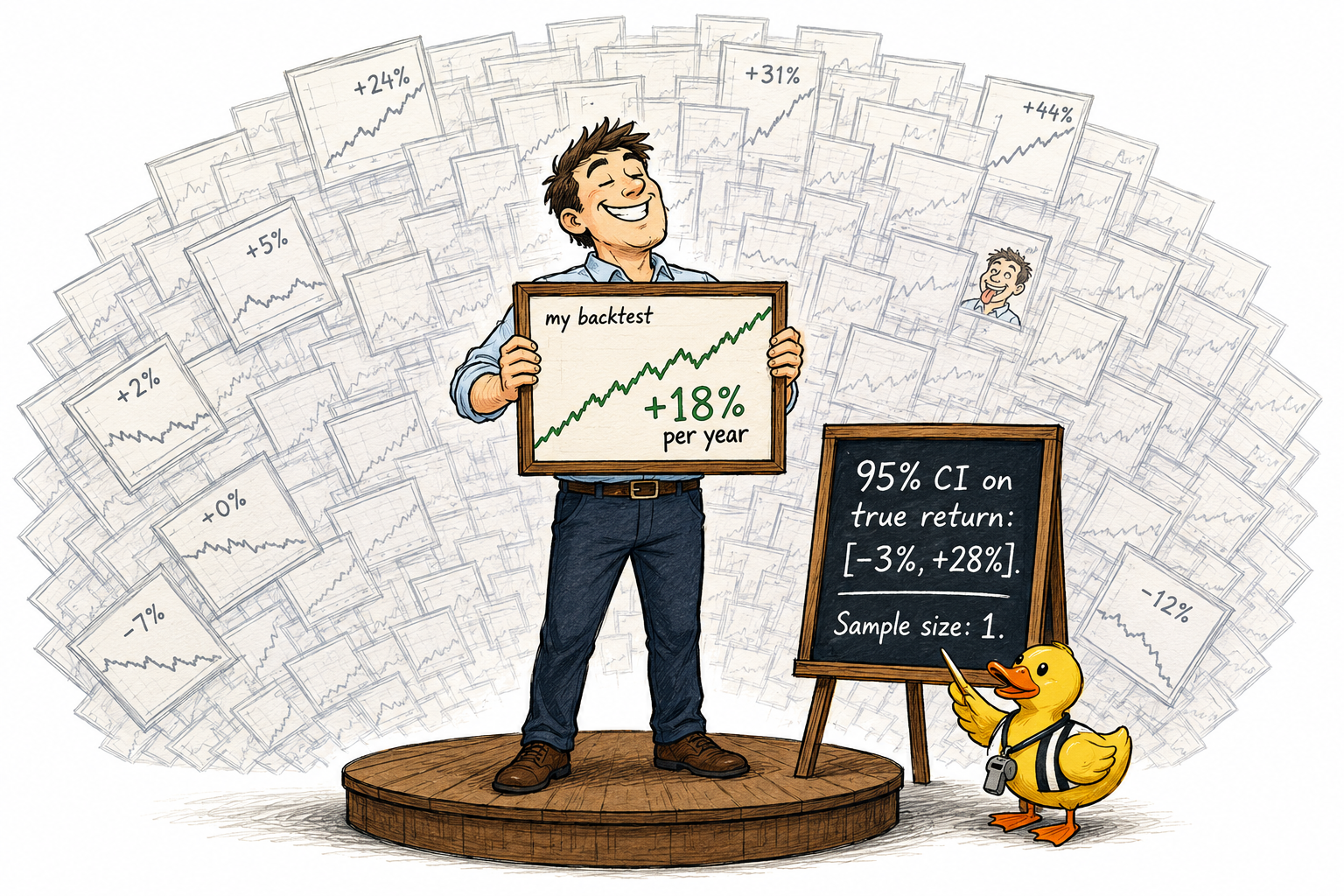
A backtest is a single draw from a distribution of possible outcomes. The number that comes out of it (annualized return, Sharpe ratio, win rate) is a point estimate with a confidence interval attached. The interval is wide enough that the point estimate, on its own, is almost uninformative.

This is not an opinion about backtesting. It is a property of finite samples in noisy data. The math is the same math that governs polling, drug trials, and weather forecasting. The size of the standard error in trading data is the part that surprises most retail researchers when they see it for the first time.

The single-number illusion

A backtest produces one Sharpe, one annualized return, one max drawdown. Each is a sample statistic, not a population parameter. The trader who writes "this strategy has a Sharpe of 1.4" has stated the sample value as if it were the truth. The truth is "this strategy produced a Sharpe of 1.4 in this specific backtest sample, which is one of many possible samples."

The distinction is not pedantic. The distance between the sample value and the true value depends on the standard error of the estimator, and the standard error in trading data is large enough that the sample value can sit far from the truth without anyone noticing.

The standard error of the mean

Every sample statistic has a standard error. For the mean return of a strategy, the standard error is:

Where σ_R is the standard deviation of the per-period returns and N is the number of independent return observations. The 95% confidence interval on the true mean is the sample mean plus or minus 1.96 standard errors.

Worked example. A strategy generates daily returns over four years (about 1000 trading days). The sample mean daily return is 0.05% (about 12.6% annualized at 252 days per year). The sample standard deviation of daily returns is 1.0%. The standard error of the mean is:

SE = 1.0% / √1000 ≈ 0.0316%

The 95% confidence interval on the true daily mean is:

0.05% ± 1.96 × 0.0316% = [−0.012%, +0.112%]

Annualized, the 95% interval on the true mean return is approximately:

[−3.0%, +28.2%]

The point estimate is 12.6% per year. The interval says the truth could be a 3% per year loss or a 28% per year gain. Both numbers are consistent with what the backtest produced.

This is what "almost nothing" means quantitatively. The headline number is real. The uncertainty band attached to it is wider than most decisions can tolerate.

Sharpe ratio: same problem, slightly tighter

The Sharpe ratio is more stable than the raw mean, but its standard error is still large at typical sample sizes. A reasonable approximation for the standard error of the annualized Sharpe with N independent daily observations is:

With a sample annualized Sharpe of 1.0 (daily Sharpe ≈ 0.063) and N = 1000 daily observations:

SE(Sharpe_ann) ≈ √((1 + 0.002)/1000) × √252 ≈ 0.0316 × 15.87 ≈ 0.50

The 95% CI on the true annualized Sharpe is approximately:

1.0 ± 1.96 × 0.50 = [0.02, 1.98]

A backtest Sharpe of 1.0 is consistent with a true Sharpe close to zero or close to two. The point estimate by itself does not distinguish these worlds. One of them is a strategy worth running. The other is a strategy that will refuse to deliver in live trading.

The window-shift experiment

Take any published rule. Run it on 2000 to 2010. Note the result. Now run it on 2000.5 to 2010.5 (shift the window by six months). Note the new result.

The two results almost never match. The Sharpe might move from 0.9 to 1.4 or from 1.2 to 0.6. The annualized return might shift by 30 percentage points in either direction. The maximum drawdown might double or halve.

The rule did not change. The data source did not change. The parameter set did not change. The only thing that changed was the slice of history that happened to be sampled.

This sensitivity is not a flaw in the rule. It is a property of the data. Market returns have high noise relative to mean, and any sample of finite length lands somewhere on the sampling distribution of possible outcomes. Different windows land in different places.

The window-shift experiment is the simplest demonstration that one backtest result is unstable.

Visualizing the sampling distribution

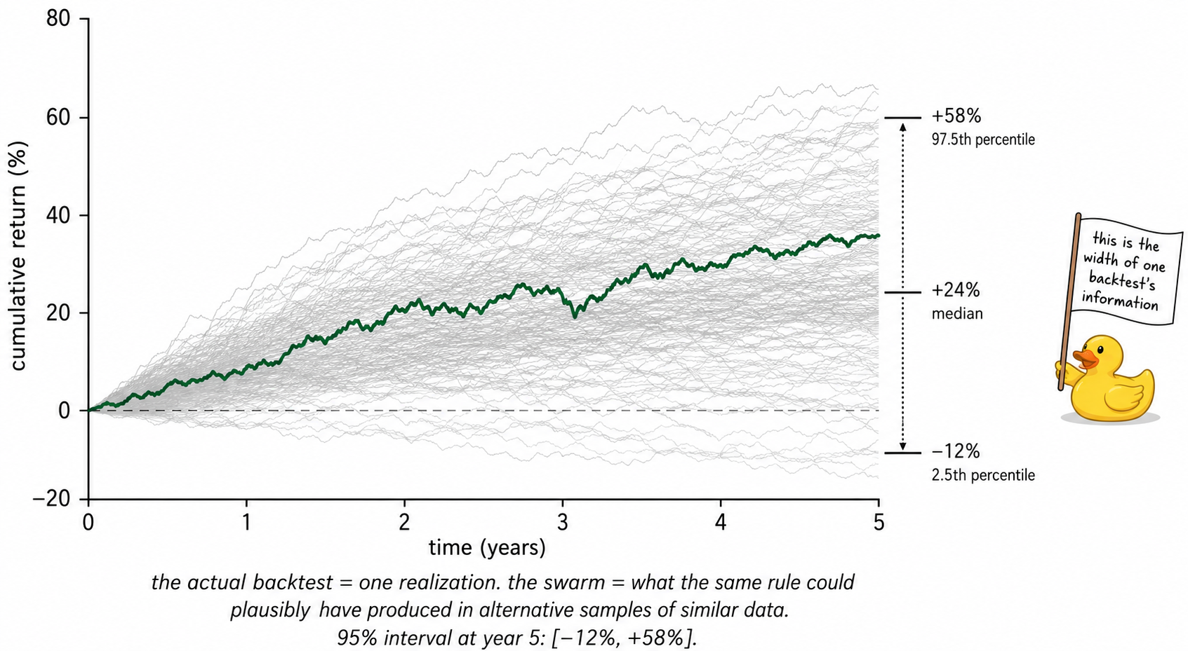
The bold curve is what gets posted on social media. The fan is what would happen if the same rule could be run on alternative draws of the same underlying process. The fan is the truth about what one backtest tells the researcher.

The block bootstrap solution

The window-shift experiment is informative but limited. It only gives a few samples. The block bootstrap gives thousands.

The procedure. Take the daily returns of the backtest. Cut them into blocks of length L (typically 5 to 20 days, long enough to preserve autocorrelation and volatility clustering). Resample the blocks with replacement until the new return series has the same length as the original. Run the strategy metric (mean, Sharpe, drawdown) on the resampled series. Repeat 5000 times.

The resulting 5000 metric values are an empirical estimate of the sampling distribution. Take the 2.5th and 97.5th percentiles to get a 95% confidence interval. Compare this interval to the headline backtest number. The gap between the point estimate and the interval edges is the size of "almost nothing."

For most retail rules the gap is enormous. For a few rules it is small enough to support a decision. Those are the rules worth running.

Why the interval is so wide

Three factors drive the width.

1. Return-to-noise ratio. The daily Sharpe of a good strategy is around 0.05 to 0.10. The daily volatility dwarfs the daily mean. Distinguishing signal from noise requires many observations.
2. Sample size. A four-year daily backtest has roughly 1000 observations. That is small by statistical standards. Polling firms reject sample sizes that small for far less noisy questions.
3. Autocorrelation and regime structure. Market returns are not independent draws. Volatility clusters, regimes persist, and effective sample size is smaller than nominal sample size. Five years of daily data has nominal N = 1260 but effective N closer to 250 to 500 once dependence is accounted for. The standard error formula assumes independence, so the naive interval is already optimistic.

The combination of these three factors makes single-backtest evidence weak in a way that is mathematical, not behavioral.

What this changes operationally

Stop reporting backtest results as single numbers. Always report a confidence interval. "Sharpe 1.2 with 95% CI [0.4, 2.0]" is honest. "Sharpe 1.2" is misleading.

Stop comparing strategies on point estimates. Compare them on intervals. Strategy A with Sharpe 1.0 and CI [0.6, 1.4] is more credible than Strategy B with Sharpe 1.4 and CI [−0.1, 2.9], even though B's point estimate is higher.

Stop concluding from a single backtest. The unit of inference is the sampling distribution, not the sample.

Use longer histories where the rule is plausibly stationary, or use higher-frequency data where more observations exist per unit calendar time. Both shrink the standard error. Walk-forward testing across multiple non-overlapping windows generates multiple samples and exposes the spread between them, which is the same information from a different angle.

KEY POINTS

• A backtest is one realization from a distribution of possible outcomes. The output statistics (mean return, Sharpe, drawdown) are sample estimates with standard errors, not population truths.
• The standard error of the mean is SE = σ / √N. For typical strategies with daily data and a few years of history, the 95% confidence interval on annualized return spans tens of percent.
• A backtest showing 12.6% annualized return on 1000 trading days with σ_daily = 1% has a 95% CI of approximately [−3%, +28%] on the true annualized mean. The point estimate carries little information by itself.
• The Sharpe ratio is more stable than the raw mean but still has a large standard error. A sample annualized Sharpe of 1.0 on N = 1000 daily observations is consistent with a true Sharpe close to zero or close to two.
• Shifting the test window by six months on the same rule and the same data source produces a substantially different result. This sensitivity is a property of noisy data, not a flaw in the rule.
• The block bootstrap reconstructs the sampling distribution of any backtest metric. Resample blocks of the original returns with replacement, recompute the metric thousands of times, and take percentiles for a 95% interval.
• Three factors widen the interval: low return-to-noise ratio in markets, small effective sample sizes in typical backtests, and autocorrelation that further reduces effective N.
• Always report confidence intervals next to point estimates. Compare strategies on intervals, not on headline numbers. The unit of inference is the sampling distribution, not the sample.