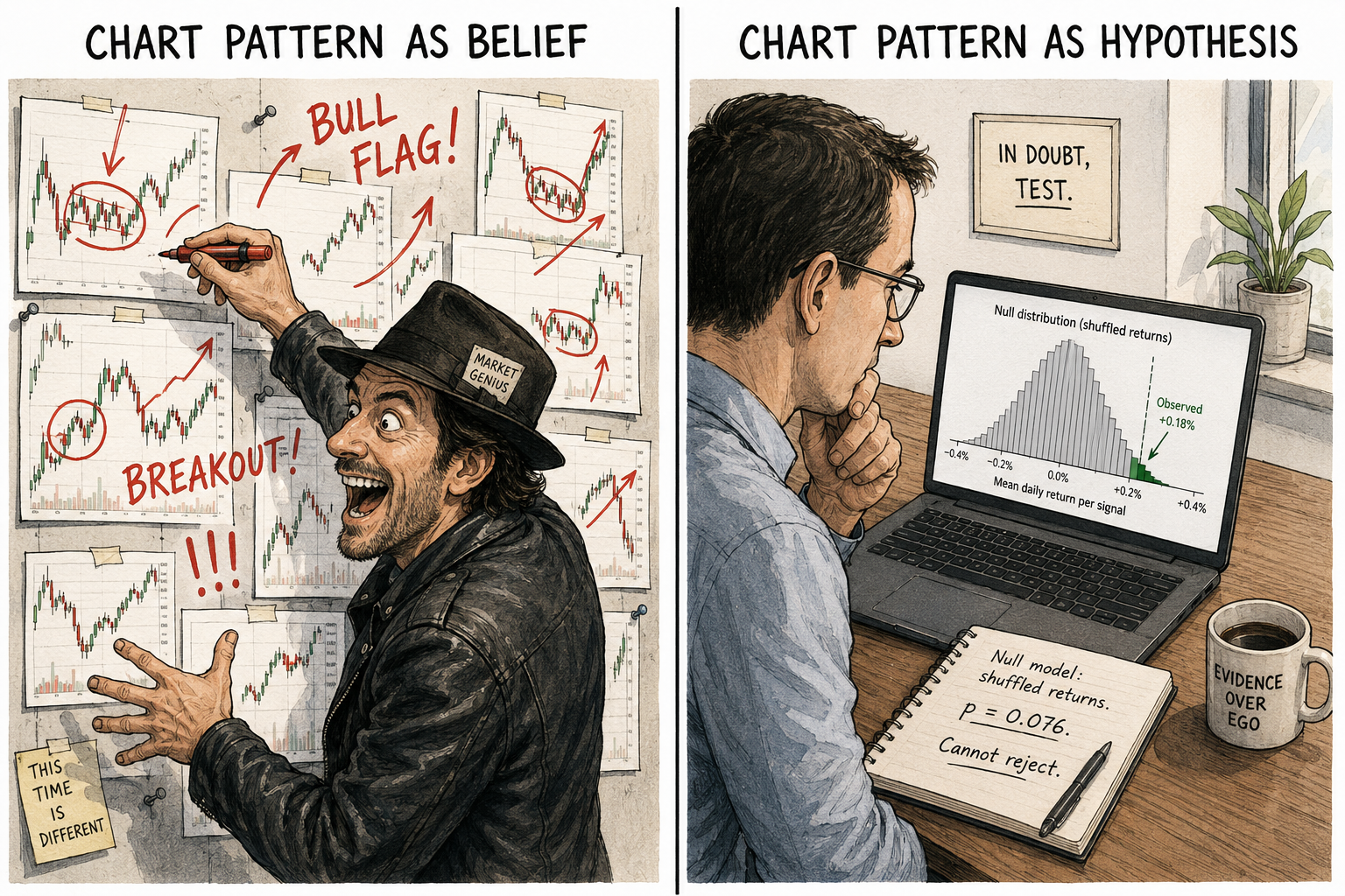
A trading rule is a hypothesis. The claim "buying when the 200-day moving average is crossed from below produces positive 7-day forward returns" is a falsifiable statement about market behavior. The market either supports it or refutes it. The trader's job is to set up the test correctly and let the data speak.

Most retail technical analysis fails to be scientific because the practitioners do not test the patterns as hypotheses. A chart with an arrow drawn on it is a claim. Without a defined test statistic, a null model, and a rejection threshold, the claim is unfalsifiable. Unfalsifiable claims sit outside the domain of evidence. They are vibes.

Three properties of a hypothesis

A scientific hypothesis has three properties.

It is specific. "Markets trend" is not a hypothesis. "The mean 5-day forward return after a positive 50-day return on the SPX from 1990 to 2024 is greater than zero" is a hypothesis. The first cannot be tested. The second can.

It is falsifiable. There must exist an observable result that would make the hypothesis false. For a trading rule, the observable result is the backtest performance. If the backtest performance is statistically indistinguishable from what the same rule would produce on data with no underlying structure, the hypothesis is rejected.

It has a quantitative prediction. The rule predicts something measurable: mean return per signal, Sharpe ratio, or hit rate above some threshold. The prediction is what you test.

A rule that lacks any one of these three properties is a description, not a hypothesis. Descriptions sit outside the domain where evidence applies.

There is only one hypothesis test

Most introductory statistics courses teach hypothesis testing as a zoo of named tests. T-test for means, chi-squared for proportions, F-test for variances, ANOVA for groups, Kolmogorov-Smirnov for distributions. Each test comes with its own table, its own assumptions, its own degrees of freedom rules. The framework underneath is the same.

The single framework, written out:

In plain words. δ_observed is a number computed from your actual data, the test statistic. It might be the rule's mean return, its Sharpe ratio, or any other property you can compute on a backtest. δ_simulated is the same number computed on a synthetic dataset generated under the null hypothesis. H₀ is the model of the world where the rule has no edge. The p-value is the probability that random data alone produces a test statistic at least as extreme as the one you saw.

Five steps make this concrete.

1. Compute the test statistic on the real data. Get one number, δ_observed.
2. Define a null model. The model has to be capable of generating fake datasets that look similar in structure to the real one but contain no signal. For a TA rule, the standard null model is the rule applied to a randomly shuffled or bootstrap-resampled version of the original return series.
3. Generate many fake datasets from the null model. A few thousand is enough.
4. Compute the same test statistic on each fake dataset. You now have a distribution of test statistics under H₀.
5. Count the fraction of fake test statistics that are at least as extreme as δ_observed. That fraction is the p-value.

If the p-value is below your threshold (the standard threshold is 0.05), the data is hard to explain under the null model, and you reject the null. If the p-value is above the threshold, you cannot reject the null, which means you cannot claim the rule has edge.

Every named statistical test is a special case of this procedure with a particular choice of test statistic, a particular choice of null model, and an analytical shortcut for computing the p-value. The shortcuts were necessary when computers were slow. They are not necessary now. Direct simulation of the null is more flexible, more transparent, and forces you to specify what you believe about the world instead of inheriting it from a textbook.

Visualizing the test

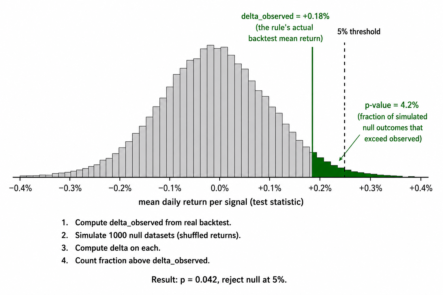
The visual shows the entire framework in one image. The bell shape is the distribution of what the test statistic looks like when the rule has no edge. The vertical line is what your rule produced. The shaded tail is the p-value. The dashed line is the threshold you committed to before you ran the test.

Applying it to a real TA rule

Take a concrete rule. "Long the SPX for 7 days after the 50-day moving average crosses above the 200-day moving average." Run it from 1990 to 2024.

Step 1. Compute the test statistic. The mean 7-day forward return after the cross signal is +0.42% across all signals in the historical sample. That is δ_observed.

Step 2. Define the null model. The null hypothesis is that the cross signal carries no predictive information. To generate fake datasets, take the historical SPX returns and shuffle them randomly to break the time structure. The shuffled return series has the same distribution as the real one (same mean, same volatility, same fat tails) but no temporal pattern. Apply the same MA cross rule to the shuffled series.

Step 3. Generate 5,000 shuffled return series and apply the rule to each. For each, compute the mean 7-day forward return after a signal.

Step 4. Plot the 5,000 mean returns. You have an empirical distribution of what the rule produces under the null. The distribution is centered near zero, with some spread due to the random shuffling.

Step 5. Count the fraction of those 5,000 means that are ≥ +0.42%. Suppose 380 of them are. The p-value is 380 / 5000 = 0.076.

That p-value is above 0.05. The rule's observed performance sits inside what the null model can produce by chance. You cannot reject the null. The "edge" you saw might be real, but the data does not support that claim at the standard threshold. The rule is not falsified, but it is not validated either.

This is the result that most retail-shared TA rules produce when tested with the right protocol. The pattern looks good on a chart. The performance looks good on a backtest. The hypothesis test says "this might be luck."

Operational consequences

Three operational consequences follow from treating a rule as a hypothesis.

The hypothesis is stated before the test. You write down the rule, the test statistic, the null model, and the rejection threshold in a file. Then you run the test. The file is timestamped. You do not get to retrofit any of those choices after seeing the result.

The null model is explicit. The shape of the null model affects the result. A naive null where returns are independent identically distributed normals will reject more rules than a realistic null that preserves the autocorrelation and volatility clustering of the original series. Choosing the more realistic null is harder and produces fewer "wins." It also produces fewer false positives in live trading.

The result has a confidence interval, not a point estimate. The same simulation procedure that generates the p-value also generates confidence intervals around the test statistic. A backtest mean return of +0.42% with a 95% confidence interval of [−0.15%, +1.0%] means something different from the same mean with an interval of [+0.30%, +0.55%]. The point estimate is the same in both, but the first is uncertain and the second is decisive. Report both.

The catch: data mining bias

The procedure above tests one specific, pre-committed rule. It does not protect against testing many rules and picking the best.

If you test 100 rules, each at a 5% significance level, around 5 will appear "significant" by chance alone, even when none of them have edge. The p-value of the best rule in a 100-rule competition is meaningless without a multiple-testing correction. The proper procedure is to either lower the threshold (Bonferroni correction divides α by the number of tests) or simulate the entire multiple-testing process (the bootstrap-reality-check family of methods).

Most retail "I tested this rule and it works" claims come from undisclosed parameter sweeps that test thousands of combinations. The reported p-value is the p-value of the best rule, not the p-value of the procedure that produced the best rule. The two differ by orders of magnitude.

KEY POINTS

• A trading rule is a hypothesis when it is specific, falsifiable, and produces a quantitative prediction. Anything less is a description.
• All hypothesis tests reduce to one framework: compute a test statistic on real data, simulate the null model many times, count what fraction of simulations produce a test statistic at least as extreme as observed.
• The framework is p = P(δ_simulated ≥ δ_observed | H₀). Every named test (t-test, chi-squared, ANOVA) is a special case with a particular test statistic and a particular null model.
• For trading rules, the standard null model is the rule applied to a randomly shuffled or bootstrap-resampled version of the return series. Shuffling breaks the time structure while preserving the marginal distribution.
• The rule, test statistic, null model, and rejection threshold must be written down before the test runs. Retrofitting any of them invalidates the result.
• Report confidence intervals alongside p-values. A point estimate without an interval is a non-answer.
• The single-test framework protects against luck in one pre-committed test. It does not protect against testing many rules and picking the best. Multiple-testing correction is mandatory when more than one rule is tested.