5.58 Retail Buys the Dip — and Destabilizes
Retail dip-buying in US equities: fit a loss slope and a gain slope on past returns. The loss slope is about -1.35, the buy arrives one period late, and a larger retail share raises volatility.
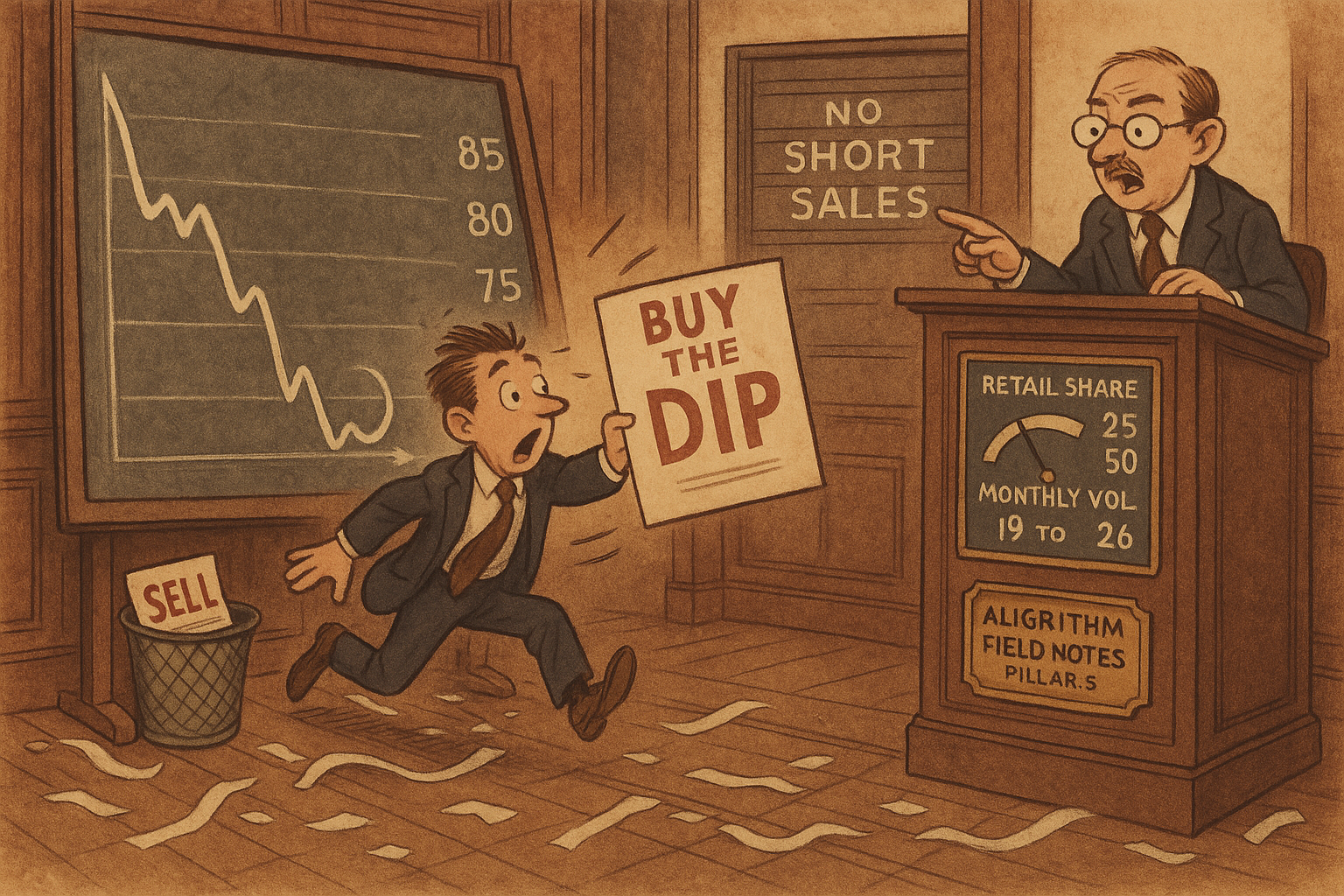
Yin and Zou take US equities from January 2017 through December 2024 and build monthly retail order flow from actual executions covering about 80 percent of US retail volume. The investor marks the stock off last period's price forecast, so a drop still looks cheap against the old anchor, and flow rises after losses. A short-sale constraint cuts off the sale after a gain, and the gain-side slope sits near zero. The buy arrives one period after a supply shock, once the price has already started back, and it pushes the price through the level it is returning to. Moving that investor from 25 percent of the book to 50 percent lifts the model's monthly return volatility from 19 percent to 26 percent.
Net flow is shares bought minus shares sold
Monthly retail net flow averages 0.232 percent of shares outstanding. The median is 0.010 percent, so the typical stock-month is a wash, and the standard deviation is 2.325 percent. The positive mean is a small accumulation over eight years.
$$ \text{RetailFlow}_{i,t} = 100 \times \frac{\text{BuyShares}_{i,t} - \text{SellShares}_{i,t}}{\text{SharesOutstanding}_{i,t}} $$
BuyShares and SellShares are that month's retail executions in the S&P Retail Flow Database, summed from the daily prints. Dividing by shares outstanding puts a 100-share name and a billion-share name on one scale, and the 100 turns the ratio into percent. On a stock with 100 million shares, the sample-mean flow is 232,000 net shares bought: 232,000 divided by 100,000,000, times 100, equals 0.232.
They keep a stock-month when the price is at least one dollar, market equity is positive, and the absolute value of this ratio is at most 1. That last cut drops a month whose net retail flow exceeds the share count. The panel that survives has 7,432 stocks over 96 months, 4,349 names a month on average, 417,519 stock-months in total. The paper does not say whether a name that leaves CRSP stays in the retail database, so this is the merged sample they describe.
Fit one slope on losses and another on gains
A 1 percentage point drop in this month's return lines up with 1.35 basis points of extra retail flow. The slope on a gain, once idiosyncratic volatility and the other controls are in the regression, is -0.06, and its standard error is 0.31.
$$ \text{RetailFlow}_{i,t} = a_t + b_i + \beta^- \min(r_{i,t}, 0) + \beta^+ \max(r_{i,t}, 0) + \varepsilon_{i,t} $$
You split the month's return r at zero. The min term is the loss, and it is zero in an up month. The max term is the gain, and it is zero in a down month. The month fixed effect and the stock fixed effect pull out that month's average flow and that stock's average flow, so the slopes are within stock. The full regression adds the same split on lagged windows, from the previous month out to the previous twelve, plus controls. Standard errors are clustered by stock and by month.
The figure annotates the single-horizon loss slope on this month's return at -1.35, with a standard error of 0.26. Single-horizon means that window alone, plus the controls, without the other windows in the same fit. A return of -0.01 changes flow by -1.35 times -0.01, which is 0.0135 percentage points of shares, or 1.35 basis points. Their prose rounds the same slope to about -1.3 and the flow response to roughly 1.3 basis points.
The fullest specification, 285,742 stock-months, puts the loss slope at -1.467, which they multiply as 1.47. The dispersion of stacked stock-month returns is 0.228. A loss of that size changes flow by 1.47 times 0.228, which is 0.335 percentage points of shares. They round that product to 0.34. Against the flow standard deviation of 2.33, 0.335 divided by 2.33 is 0.144, and they call it roughly 14 percent of a typical month's flow dispersion. The prose calls this return dispersion 22.75 percent. The table prints 0.228, and 0.228 is the number in the product.
The gain slope in that same specification is -0.057, standard error 0.307. A 10 percent up month changes fitted flow by -0.057 times 0.10, which is -0.0057 percentage points. With no controls and only the current month, the gain slope is +1.904, so the same up month lines up with 1.904 times 0.10, or 0.19 percentage points of extra flow. The single-horizon fit, controls in and the other windows out, puts that gain slope at -0.06 with a standard error of 0.35. Idiosyncratic volatility, the 21-day standard deviation of the residual from the market, size, and value factors, has a coefficient of 22.663. Its own standard deviation is 0.033, so a one-standard-deviation move lines up with 22.663 times 0.033, which is 0.748 percentage points of flow, against 0.335 from the one-standard-deviation loss. The skewness coefficient is -0.039. Holding volatility fixed, flow is a bit lower when that residual is right-skewed.
Read the left panel. Every loss slope is negative. The right panel is the gain side, and it sits on zero.
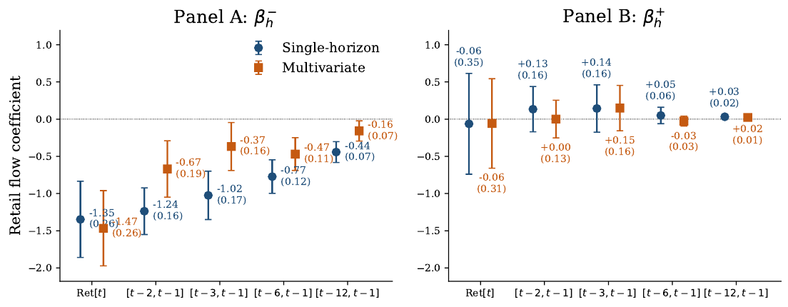
The orange squares are the joint regression. At the current month the joint loss slope is -1.47 and the single-horizon loss slope is -1.35, so the joint estimate is the larger of the two. Their sentence that every joint loss slope is smaller in magnitude than its single-horizon pair does not hold on this month. It does hold on the lagged windows, where the joint slopes are -0.67, -0.37, -0.47, and -0.16.
The twelve-month loss coefficient in the table is -0.158. A stock down 50 percent over that window, a return of -0.50, draws -0.158 times -0.50, which is 0.079 percentage points of extra retail flow in each month the window still looks like that. They round the coefficient to -0.16 and the flow to 0.08. The twelve-month gain coefficient is 0.023 with a standard error of 0.013, the one gain slope with a 10 percent star, and a 50 percent rally draws 0.023 times 0.50, which is 0.012 percentage points. The within R-squared of the full regression is 0.09. The kink is estimated tightly, and it leaves most of the month-to-month flow unexplained.
Past-twelve-month losers lead in 97 percent of months
Sort each month on the return from twelve months ago through last month, and the bottom third receives 0.47 percent of shares in retail net flow. The middle third receives 0.05 percent. The top third receives 0.10 percent.
$$ \text{Gap} = \overline{\text{Flow}}_{\text{bottom}} - \overline{\text{Flow}}_{\text{top}} $$
The gap is the average flow of the worst third minus the average flow of the best third, each average taken across the 96 months. 0.47 minus 0.10 is 0.37 percent of shares, with a t-statistic of 6.45. The bottom third's flow exceeds the top third's in 97 percent of months. The autocorrelation of that bottom-third series is 0.67, so a heavy month for losers tends to be followed by another. The months that break the ordering cluster in the meme-stock window of early 2021, when flow into recent winners jumped. That window is the attention episode in the old article "Is Attention a Factor? WSB Herding, BERT Sentiment, and the Meme Confound". The ordering comes back after it, and it holds through the COVID selloff from February to May 2020. They also weight each third by market cap. That version is described, the averages are not reprinted, and the shape is the same.
Total initiated flow, the rest of the tape, runs the other way. In the same past-return thirds it averages -0.69 percent of shares in the bottom third and -0.33 percent in the top third. The gap is -0.69 minus -0.33, which is -0.36 percent, with a t-statistic of -4.06. Retail is buying the names the rest of the tape is selling. Net flow in prints above 50,000 dollars slopes the same way: buyers of past winners, sellers of past losers. The change in lendable supply slopes that way too, and so does the quarterly change in 13-F ownership.
The paper also says the bottom third of total flow lies below the top third in only 9.4 percent of months. A mean gap of -0.36 and a month-count of 9.4 percent sit together only if a minority of months carries the average. The retail line next to it is "ahead in 97 percent of months," and 100 minus 9.4 is 90.6, so the 9.4 percent sentence may have the complement backwards. Keep both numbers as printed. Use the -0.36 mean. Recompute the month count before you treat 9.4 percent as a frequency.
Sorting on this month's return mixes the flow with the same month's volatility. Retail flow is then 0.37 percent in the bottom third, 0.05 in the middle, and 0.26 in the top. They print the bottom-minus-top gap as 0.10 with a t-statistic of 4.09. The printed averages subtract to 0.37 minus 0.26, which is 0.11, so the 0.10 is a rounded gap. The bottom third leads in 74 percent of months. This month's return is set in the same month as the flow, and the up-month names are the high-volatility names from the regression above. The lagged window is already finished when the flow arrives.
The net slope is the buy slope minus the sell slope
Gross buying and gross selling both load near -12 on a lagged loss. The net slope left after you subtract them is -1.24.
$$ \beta^-_{\text{net}} = \beta^-_{\text{buy}} - \beta^-_{\text{sell}} $$
Net flow is gross buying minus gross selling, so the loss slope on the net has to equal the loss slope on buying minus the loss slope on selling, in the same regression. At the one-month lagged horizon those gross slopes are -12.54 and -11.30, with standard errors near 3.9. Then -12.54 minus -11.30 equals -1.24, and the standard error on the net is 0.16. The paper calls that drop in the standard error roughly twenty-five-fold. 3.9 divided by 0.16 is 24.4.
A lagged return of -0.10 raises gross buying by -12.54 times -0.10, which is 1.254 percent of shares, and gross selling by -11.30 times -0.10, which is 1.130 percent of shares. The net left over is -1.24 times -0.10, which is 0.124 percent of shares. Both sides of the retail tape get louder when the past move is large, on either side of zero, and market turnover traces the same shape. The dip-buy is the wedge that remains after that common spike cancels.
The old article "Why Traders Take Profits Too Early and Losses Too Late" describes the disposition effect, in which selling slackens after a loss because the holder will not realize it. The sell slope here is -11.30, the same sign as the buy slope, and almost the same size. The old article "Get-Even-Itis: The Most Expensive Disease in Trading" is the urge to add to a loser until the position is whole. The net flow does add to losers. The gross legs say the tape also sells more of them. The object on this tape is a turnover spike with a contrarian remainder.
Today's price gets a 1 percent weight
The price retail acts on puts a 0.01 weight on the live print and a 0.99 weight on last period's forecast.
$$ \tilde{p}_t = m\, p_t + (1 - m)\, \hat{p}_t $$
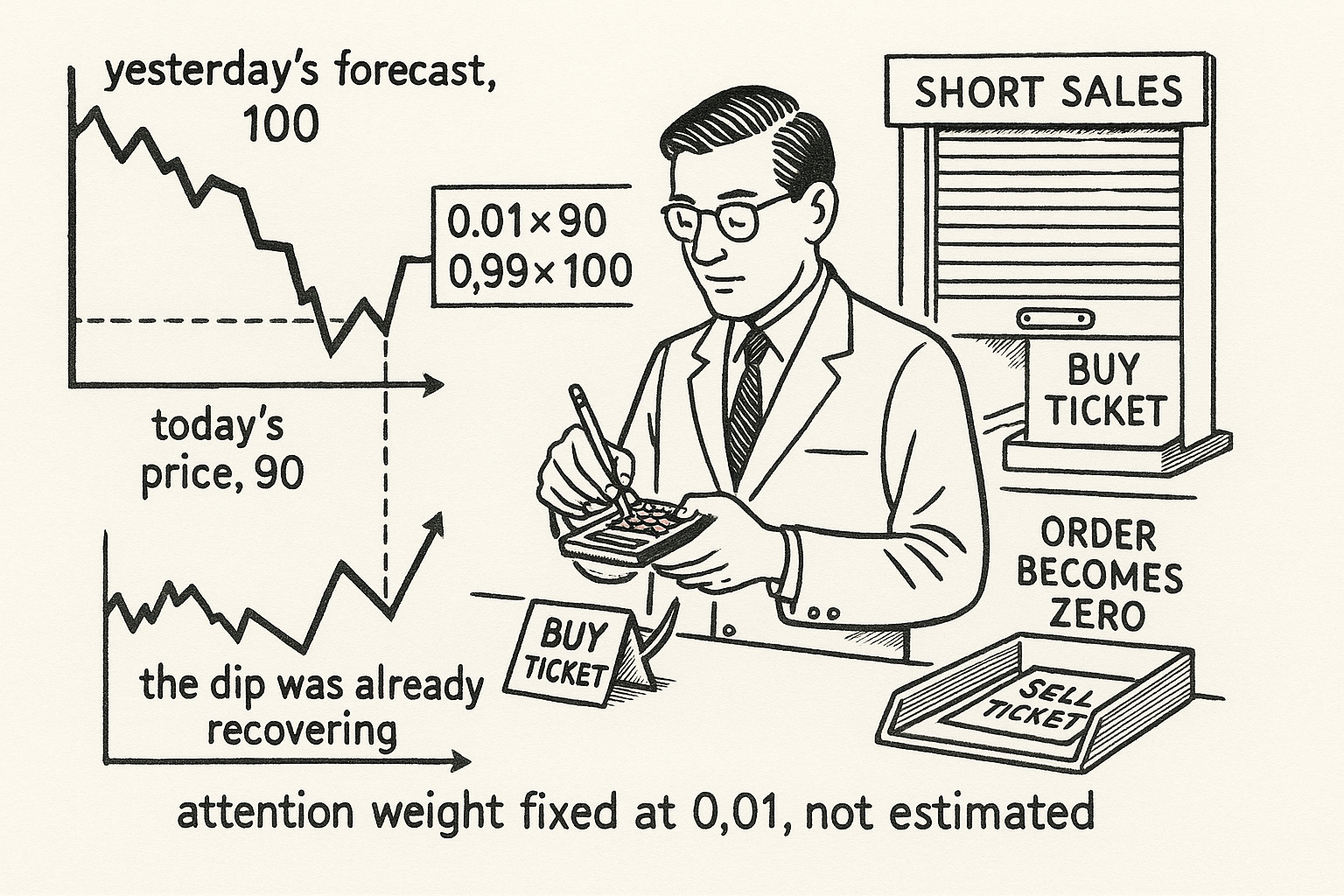
p is the price cleared this period. The forecast next to it is retail's expectation of that price, formed from information through last period. m is the weight on the live price. They fix m at 0.01 and do not estimate it. Suppose the forecast is 100 and the market has fallen to 90. The marked price is 0.01 times 90 plus 0.99 times 100, which is 0.9 plus 99, which is 99.9. Retail is marking a price of 90 at 99.9, and that gap is a buy. The anchor updates after the trade, from the price and the cash flow realized this period, so the buy shows up next period and is absent in the shock period.
$$ q_{i,t} = \max\{\tau^R (\mu_t^R - \tilde{p}_t) - h_i,\ 0\} $$
Tau-R is retail risk-bearing capacity, mu is retail's forecast of the next cum-dividend payoff, and h is a hedging need that differs across retail investors. The term inside the max is the position they would hold with no constraint. After a rally the stale mark sits high, that position is a short, and the max with zero deletes it. A desired position of -2 becomes an order of 0. A desired position of +2, the dip, goes through as +2. Institutions have no such cap. Sparse attention on its own gives you a contrarian schedule on both sides of zero. The constraint on its own gives you a flat schedule. The loss-side buy and the flat gain side show up when both are on.
Aggregate demand integrates that max over a normal cross-section of hedging needs. They set the dispersion of those needs to one millionth, and at that width the integral is a hard kink: positive demand passes through, negative demand is zero. They fix the dispersion. The estimated hedging level is 10.153, and it shifts the whole schedule up or down. A 10 percent change in it moves the level and leaves the curvature alone.
The paths are scored on a second regression, with no stock or month fixed effects. Flow and the lagged return are in decimal units, and simulated flow is rescaled until its standard deviation equals 0.014.
$$ Q_t^R = a + \beta^- \min(r_{t-1}, 0) + \beta^+ \max(r_{t-1}, 0) + u_t $$
This is the regression on the simulated paths. The loss slope is -0.031 in the data and -0.031 in the model. A lagged return of -0.10 changes flow by -0.031 times -0.10, which is 0.0031, or 0.31 percent. That is the "10 percent decline, 0.31 percent more flow" in the text. The gain slope is 0.008 in the data and 0.004 in the model, so a return of +0.10 changes model flow by 0.004 times 0.10, which is 0.0004, or 0.04 percent. The model understates the gain side and keeps the shape.
The panel slope of -1.35 and this -0.031 are different regressions. Divide the panel slope by 100 and you are in decimal flow units: -1.35 divided by 100 is -0.0135. Their footnote puts the fixed-effects slope, in those units, near -0.013. The -0.031 they match is the pooled slope, the one with no fixed effects. Dividing 0.031 by 0.0135 gives 2.3, so the pooled slope is steeper, and the sign is the same. Separately, Table 1's flow standard deviation is 2.325 percent, which is 0.02325 in decimal units, and the calibration pins flow volatility at 0.014. The source prints both and does not say how they differ. Keep 0.014 inside the calibration and 2.325 inside the panel. The source may be matching a different dispersion, and the page does not identify it.
The retail ticket is zero on the shock and large one period later
Retail flow is zero in the period of the shock. One period later it is about 4.9 percent after a price decline and about 0.15 percent after a rise.
$$ \tau^I = \frac{1 - \alpha}{\gamma_I \sigma_I^2}, \qquad \tau^R = \frac{\alpha}{\gamma_R \sigma_R^2} $$
Alpha here is the retail share of the book. Gamma is risk aversion. Sigma-squared is the payoff variance each side prices, and they set both variances to 1. At a retail share of 0.25 the estimated capacities are 0.103 for institutions and 1.167 for retail. Institutional risk aversion is then 0.75 divided by 0.103, which is 7.28. Capacity is proportional to one minus the retail share when that aversion stays put, so moving the share from 0.25 to 0.50 multiplies institutional capacity by 0.50 divided by 0.75, which is two-thirds. Then 0.103 times two-thirds is 0.0687. Retail capacity scales with the share, so it goes from 1.167 to 2.334. The same supply shock now hits a smaller institutional book, and the delayed retail correction is larger.
$$ \lambda_t = \rho_\lambda \lambda_{t-1} + u_{\lambda,t} $$
Lambda is transitory supply pressure, extra shares the market has to absorb. They fix its persistence at 0.5. A shock of size 2 this period is size 1 next period, before any new innovation, and size 0.5 the period after that. Cash-flow persistence is fixed at 0.96, so the state that reverts is supply, and the earnings state barely does. Retail's flow peak sits on the first of those dates, when half the supply shock is already gone.
Look at the solid line. It is a positive supply shock, and it drives the price down. The dashed line is the mirror shock.
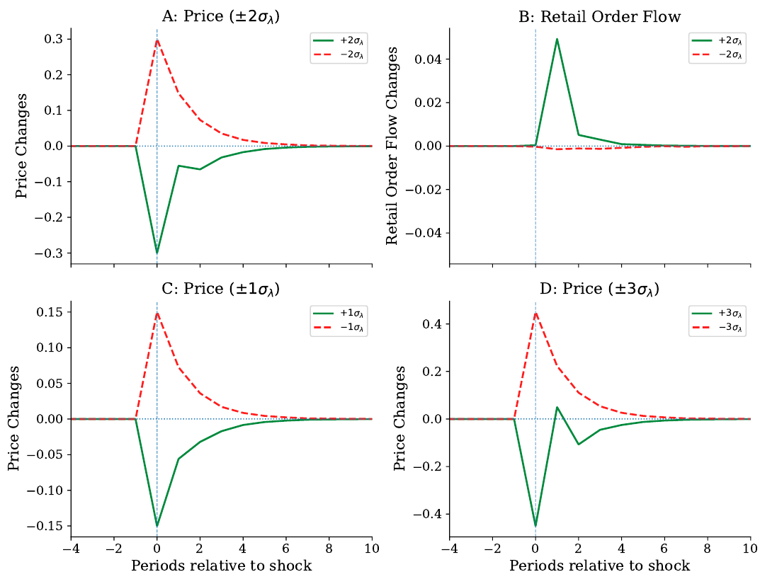
In the top-left panel a positive supply shock of two standard deviations moves the price by about 0.30 on impact, which they call about 30 percent, and the dashed line moves about 0.30 the other way. Impact is symmetric, because institutions are the only ones trading and their demand is linear. In the top-right panel retail flow is flat at the shock date. One period later the solid line, the dip, peaks near 0.05, and they read that peak as about 4.9 percent more retail flow. The dashed line, the rally, moves by about 0.15 percent. Dividing 4.9 by 0.15 gives 33, on those rounded readings. The price path after the dip snaps most of the way back in that same period, sags again once the buying normalizes, and settles through a damped wobble. The path after the rally decays smoothly, near the supply state's own rate of one-half per period. In the bottom-right panel the larger dip, three standard deviations, crosses back above zero before it settles. A buyer who arrived on impact would have leaned against the shock. This buyer arrives the next period, into a move that is already on its way back.
That delay is loaded on the attention weight of 0.01. Raising the weight to 0.10 or 0.30 flattens the loss-side flow schedule, because retail then sees the live price and the extra buying lifts that price inside the same period. They do not reprint the volatility chart at those higher weights. The share experiment below is the near-zero-attention model.
The volatility line the calibration did not target
Look at the solid line in the left panel. It is the model's monthly return volatility against the retail share, and the calibration was not asked to match it.
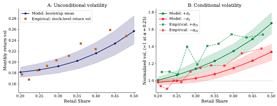
The paper reads that line as about 19 percent at a 25 percent retail share and about 26 percent at 50 percent. On the right, volatility after a positive supply shock sits above volatility after a negative one, and they say the gap widens from about 13 percent at a share of 0.25 to 30 percent at 0.50, with both series scaled to 1 at the low-shock value when the share is 0.25. The squares and the dashed lines are stock-level volatility binned by retail share; the high-pressure bin is a lagged forced-flow score one standard deviation above its monthly mean, and the paper says those squares stay inside the shaded band over most of the range, while the calibration matches a loss slope of -0.031 on both sides, a gain slope of 0.004 against an empirical 0.008, and a baseline return volatility of 0.183.
That 0.183 is 18.3 percent. The abstract's 19 percent is their rounding of it. Table 1's 0.228 is the dispersion of stacked stock-month returns, which is wider than the average stock's own volatility, and the squares in the figure live near 0.19 at a low retail share. 26 divided by 19 is 1.37, so the rounded pair is about 37 percent more volatility, and both inputs are already rounded.
The right-hand empirical series is not a slope sitting in a table you can recompute. The pressure score counts mutual funds forced to sell a stock against funds forced to buy it, divided by the number of prior holders, lagged a month, and the volatility is the later one. You need the fund-flow file to build it. They treat a high positive score as the empirical cousin of a positive supply shock.
Widen into the period after the drop
I am against joining that buy. It is late, volatility on the share chart rises with the retail share, and the paper never shows the holding-period return. Aggregate flow has no exit, no spread, and no borrow. Whether that ticket earns a reversal after costs is the question they leave open. There is no cost number to haircut, because there is no strategy on the page.
If you quote, the state is the retail share and the sign of recent supply pressure. On the shock itself, institutions take it and the price move is roughly linear. Retail flow shows up the next period, about 4.9 percent on the dip against about 0.15 percent after a rise, at the attention weight they fixed. That is the period when the path overshoots, and the overshoot is larger when the shock is large. Widen, or skew the quote, into that next period when the retail share is high. They do not tell you the spread to charge. If the retail in your name watches the live price, this calibration is the wrong one, because the volatility line was never rerun at an attention weight of 0.10 or 0.30.
Build the flow from actual retail prints. BJZZ, the sub-penny flag that calls a trade retail when the execution is off-exchange and the cent fraction sits away from zero and away from half a cent, has a time-series correlation of 0.017 with this flow. After 2021 that correlation is -0.075. BHJOS keeps the same sub-penny filter and signs the trade by where it sits inside the spread, and its time-series correlation is 0.347. The cross-section is kinder: about 0.478 for BJZZ and 0.508 for BHJOS, higher among small stocks and past losers, which is the corner a dip-buy study would least like to measure badly. The month-by-month ordering above is a time series, and the flag misses the time series.
The week everyone uses as the retail case is a sell. On 26 January 2021 the GME close was 147.98, up from 76.79 the day before, and Citadel's published retail print was a net sale of 1,906,567 shares on volume of 178,587,974. Divide those shares by that volume and you get 0.0107, which is the table's -1.07 percent once the sign is restored. The next day, at a close of 347.51, the print was a net sale again. The S&P series agrees in sign from 25 January through 27 January. BJZZ sits near zero through the squeeze.
Size the loss state off the share chart, not off one monthly width. The old article "Fat Tails: Why Gaussian Thinking Breaks Trading Systems" is the case against a single Gaussian width. This model is Gaussian, and the conditional gap on the right-hand panel still widens with the retail share, from about 13 percent to 30 percent. The panel's stacked monthly return dispersion is 0.228. A size that uses one of those widths in every state is using the small one when the retail share and the supply shock are both high.
KEY POINTS
- Compute retail net flow as buy volume minus sell volume, divided by shares outstanding. The mean is 0.232 percent of shares a month, on 417,519 stock-months.
- Split the return at zero. The single-horizon loss slope on this month's return is -1.35; the gain slope in the full regression is -0.06.
- Sort on the past twelve-month return. Bottom-third retail flow exceeds the top third in 97 percent of months, and the gap is 0.37 percent of shares.
- Mark the price retail trades at 0.01 times the live price plus 0.99 times last period's forecast. A fall from 100 to 90 is still marked at 99.9.
- Do not lean on the dip-buy as a stabilizer. With attention fixed at 0.01, monthly volatility goes from about 19 percent to about 26 percent as the retail share goes from 25 percent to 50 percent, and retail flow is zero in the shock period.
References
- Is Attention a Factor? WSB Herding, BERT Sentiment, and the Meme Confound
- Why Traders Take Profits Too Early and Losses Too Late
- Get-Even-Itis: The Most Expensive Disease in Trading
- Fat Tails: Why Gaussian Thinking Breaks Trading Systems
- Buying the Dip in Retail Trading, Xiao Yin and Dongchen Zou
A note on AI. The ideas, research, analysis, and conclusions in this article are my own. I use AI tools to help with editing and wordsmithing, because English is not my first language, and I am not shy about that. AI-generated ideas and AI-assisted writing are not the same thing: the first is empty slop from a generic prompt, the second is a tool for communicating years of real research more clearly. Judge the work by its substance, not by whether software helped polish the prose.