3.53 Find the Basket, Not the Pair: Sparse Mean-Reverting Portfolios
Sparse mean-reverting swap portfolios cap how many rates you hold and minimize the variance share the lag explains. A 1bp spread flattens the Sharpe; dense books often sit inside the bid-ask.
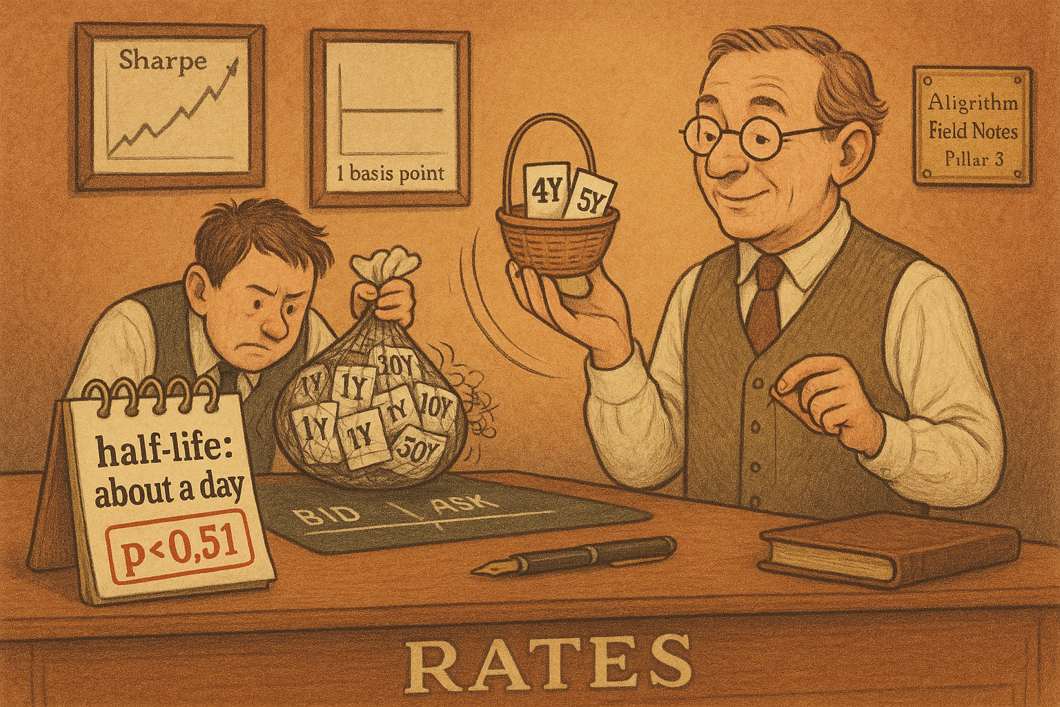
d'Aspremont caps the Box-Tiao decomposition. That decomposition ranks portfolios by the share of today's variance that yesterday already explained, and the cap limits how many assets may carry a nonzero weight. On US swap rates the printed two-name basket is the 4-year at -0.714 and the 5-year at 0.700. Leave the cap off and the solution holds every maturity on the curve. A dense portfolio costs more to trade, is harder to read, and often oscillates inside the bid-ask spread, so the capped problem is a sparse generalized eigenvalue problem.
Minimize the share of variance the lag already explains
A basket is a weight vector x on the levels. Its predictability is the share of its variance that sits in the lagged basket. d'Aspremont uses a small share as the proxy for fast mean reversion, and a large share as the proxy for momentum. The letter he uses for that share collides with the letter he later uses for reversion speed, so here the share is ν and the speed, defined below, is λ.
$$ \nu(x) = \frac{x^{\mathsf T} M x}{x^{\mathsf T} \Gamma x}, \qquad M = A^{\mathsf T} \Gamma A $$
Γ is the covariance of the levels. A is the coefficient in the regression of today's curve on yesterday's curve, so M is the covariance of the fitted part. The numerator is the variance of the part yesterday already determined. The denominator is the variance of the basket. The ratio is between 0 and 1 when the regression is a stationary fit.
Take a two-name toy with Γ equal to the identity and
M = [[0.50, 0.30], [0.30, 0.50]].
Each name alone scores 0.50, because that is the diagonal. The spread x = (1, -1) divided by the square root of 2 has squared length 1, and the quadratic form is 0.25 + 0.25 - 0.15 - 0.15 = 0.20. The sum of the two names, with the cross terms flipped, scores 0.80. Mean reversion keeps 0.20. Momentum keeps 0.80. Same two matrices, opposite end.
For a single series the share is the square of the autocorrelation. A daily autocorrelation of 0.50 means predictability 0.25: the lag accounts for a quarter of the variance, and the shock accounts for the rest. Minimizing ν pushes the basket toward that noisy end. It does not, by itself, hand you a half-life. The speeds in the swap table run from 0.58 to 238.11, which cannot be variance shares. Those are Ornstein-Uhlenbeck speeds fit after the weights are chosen.
The Ornstein-Uhlenbeck speed λ is the continuous rate in dP = λ (mean − P) dt + σ dZ. The basket level is pulled toward its mean at that rate, and σ is the diffusion. Johansen's cointegrating vectors are the same generalized eigenvalue problem run on changes against lagged levels. One ratio covers both jobs. Point the ratio up and you are hunting momentum. Point it down and you are hunting reversion.
Cap the nonzeros, then solve the small eigenproblem
The exact in-sample minimum of ν cannot rise when you allow another name. The best basket of size k+1 is at least as unpredictable as the best basket of size k, because the smaller basket is still available. Sparsity is a constraint you add on purpose. The unconstrained solution is dense, and dense is what you are refusing.
$$ \min_{x} \ \nu(x) \quad \text{subject to} \quad \mathrm{Card}(x) \le k, \quad \|x\|_{2} = 1 $$
Card(x) is the count of nonzero weights. k is the most names you will hold. The unit-length constraint kills the trivial rescaling, since the ratio does not care about scale. The paper writes the same program as a maximization. That version is the momentum basket. Mean reversion is the minimization. The paper notes the sparse version is subset selection, which is NP-hard, so you take a greedy path or a convex upper bound.
The greedy path starts at one name.
$$ i^{\star} = \arg\min_{i} \ \frac{M_{ii}}{\Gamma_{ii}} $$
Score each asset by its own predictability and keep the smallest. In the toy both names score 0.50, so the one-name book stops at 0.50 and the second name is what drops the share to 0.20. On the printed swap composition the one-name basket is the 5-year with weight 1.000. From a support of size k you try every name still outside, solve the generalized eigenproblem on those k+1 names, and append the name that lowers ν the most. Each pass costs on the order of k squared times the names still outside. A full set of cardinalities costs on the order of n to the fourth. The paper's benchmark, a full sweep on 100 names, took one minute and forty seconds.
The printed supports are nested, which this recursion forces and the true subset need not obey. The two-name basket is the 4-year at -0.714 and the 5-year at 0.700. The squared weights sum to 1.00, so the unit-length constraint is met within rounding. The three-name basket brings in the 3-year at -0.288, moves the 4-year to 0.806, and moves the 5-year to -0.517. Long the belly, short the wings, in rate space: a butterfly, where the two-name basket was only a slope. The 2-year weight stays at 0 until the seventh name, and the 7-year stays at 0 until the eighth. The path loads the belly and ignores the wings until it has nothing else to add. That is readable. It is also the failure mode of a nested search. The paper says you can run the same recursion backward, dropping the name you can spare, and it gives no suboptimality bound for the forward path. The printed table is not labeled as the backward pass. Treat it as one forward path from a window the paper does not date.
The convex alternative lifts x to X = xx-transpose, drops the rank-one constraint, and replaces the count of nonzeros with a cap on the sum of absolute entries. A k-sparse unit vector has an absolute sum of at most the square root of k, so the sum of absolute entries of xx-transpose is at most k. On the printed two-name weights the absolute sum is 0.714 + 0.700 = 1.414, and 1.414 squared is 2.00, which sits on a cap of k = 2. The semidefinite program returns an upper bound. When the solution has rank one, the bound is the answer. When it does not, you take the leading eigenvector. On the swap comparison the relaxation beats the greedy path at some middle cardinalities, the greedy path is the smoother of the two, and they meet at k = 1 and at k = 8. Keep the relaxation when you want that bound. The path you will rerun every window is the greedy one, forward and then backward.
The half-life is the natural log of two, over the speed
Once the weights are fixed, integrate the Ornstein-Uhlenbeck over one step and regress the basket on its lag. The slope φ is e to the minus λ Δt. Predictability of that univariate basket is φ squared, so minimizing ν and maximizing λ point the same way when the basket is an autoregression. The eigenvalue is a variance share between 0 and 1. The half-life comes from the speed you fit afterward.
$$ \hat\phi = \frac{\sum_{t=1}^{N}(P_t-\hat\mu)(P_{t-1}-\hat\mu)}{\sum_{t=1}^{N}(P_{t-1}-\hat\mu)^{2}}, \qquad \hat\lambda = -\frac{1}{\Delta t}\ln\hat\phi $$
The slope is the ordinary regression of today's demeaned basket on yesterday's. λ is minus the natural log of that slope, divided by the step in years. Use the natural log. A base-10 log of 2, divided by 238.11 and multiplied by 365, is 0.46 days, and that is not the "about one day" the paper states. The natural log is the conversion that reproduces the sentence.
Walk a noise-free path whose true slope is 1/2: levels 1, 1/2, 1/4, 1/8, already demeaned for the exercise. The cross product is 1/2 + 1/8 + 1/32 = 21/32. The lag sum of squares is 1 + 1/4 + 1/16 = 21/16. The ratio is 1/2, the 21 cancels, and with Δt = 1/252 the speed is 252 times the natural log of 2, which is 174.67 per year. The paper's displayed fraction puts the contemporaneous sum of squares in the denominator. On this path that sum is 21/64, the ratio is 2, and the speed is -174.67. A noise-free decaying path gets labeled as an explosion. The two denominators agree in population, under stationarity, and they do not agree on a short window. Code the lag sum of squares. That is the regression the integral describes. The displayed fraction swaps it.
The displayed volatility has two further breaks. The residual is written with today's price in both terms, so the lag never enters, and the residual sum sits outside the square root, which is the wrong dimension for a volatility. The integral line above that display is the one that matches the process. A shock over a step Δt has variance σ squared times (1 − e to the −2λΔt) / 2λ. Invert that if you need σ. Do not code the display. The source may have swapped an index; the path above shows the printed ratio is not a harmless rewrite.
$$ \tau = \frac{\ln 2}{\lambda} $$
τ is the half-life: the time for a shock to decay by half, because e to the minus λτ equals 1/2. On the noise-free path, λ = (ln 2) / Δt, so the half-life is exactly one step. One trading day, if the step is a trading day.
The paper says a mean-reversion coefficient of 238 implies a half-life of about one day. The fastest entry in the canonical table is 238.11. The natural log of 2 over 238.11 is 0.00291 years, which is 1.06 days on a 365-day year and 0.73 days on a 252-day year. Their sentence matches the calendar conversion. They do not print the day count. On the 252-day clock the sixth coefficient in that table, 174.82, is the one-trading-day portfolio: the half-life is 1.00 trading day. 238.11 stays as printed.
Zero the weak conditional links, then search inside a piece
Estimating Γ by the sample covariance and A by least squares is unstable once the curve is long, and it keeps every conditional link, including the ones that are dust. Covariance selection replaces that estimate with a precision matrix, the inverse covariance, penalized by the sum of absolute entries. A zero in the precision means the two series are independent after you condition on the rest. In rates language, the idiosyncratic moves are unrelated.
$$ \max_{X} \ \log\det X - \mathrm{Tr}(\Sigma X) - \rho \sum_{i,j} |X_{ij}| $$
Σ is the sample covariance. X is the precision. ρ is the charge per unit of absolute precision. The unpenalized optimum is Σ inverse.
Put a correlation of 0.90 on the table, variances 1, so Σ is [[1, 0.90], [0.90, 1]]. The determinant is 0.19. The precision has diagonals 5.26 and off-diagonals -4.74, and the sum of absolute entries is 20. At ρ = 0.10 the penalty, evaluated at that unpenalized fit, is 2.00. The log-likelihood term there is -0.34. The charge is the larger piece, so the penalized optimum has to shrink the off-diagonal. This ρ is not a universal knob. The paper uses 0.10 on swap rates in percent and 0.01 on dollar crosses in price levels, and it does not say it standardized Σ first. Copying 0.10 onto a book with different units is a different penalty.
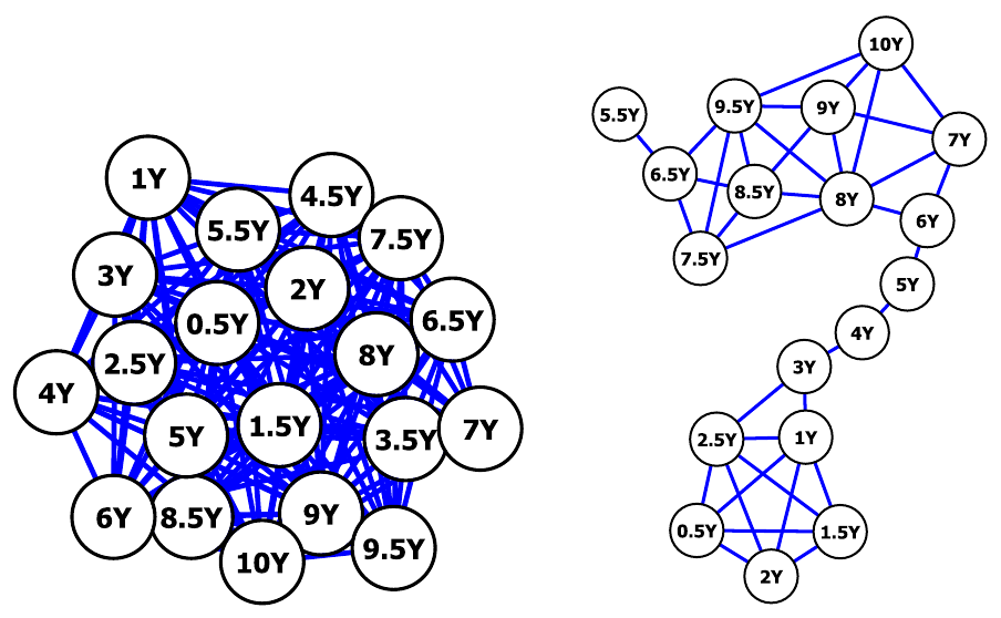
Look at the right-hand graph. Maturities that still share a conditional link sit next to each other along the curve. The left-hand graph, from the raw inverse, connects almost everything to almost everything. If the penalized precision falls into disconnected pieces, and the penalized regression for A splits on the same pieces, the support of the optimal basket lies inside one piece. You then run the greedy path inside the piece. If the graph stays connected, the theorem does not fire, and you search the whole set. The old article "Stat-Arb Is a Clustering Problem: Multi-View Spectral > Any Signal" is the later, heavier version of the same order of operations: decide who belongs together before you hang a signal on the group. Covariance selection is the cheap Gaussian cut that comes first.
On the dollar crosses the paper runs that cut with ρ = 0.01, keeps a cluster of fourteen, and also penalizes the regression for A hard enough to zero 20% of the coefficients. The drawn cluster has Sri Lanka and Hungary in the middle and includes Finland. The universe also lists Eurozone, and the sample starts in April 2002, three years after Finland adopted the euro. The paper does not say how those two dollar rates differ. The bid-ask figure it quotes, about 0.0005, is for key rates. Sri Lanka is not a key rate. A spread measured on the euro does not describe the cluster the penalty returned.
Out of sample, extra names buy speed and sell range
On US swaps from 1998 to 2005 the greedy path is refit on windows of 200 days, stepped every 50 days, so neighboring windows share 150 days. The paper plots the average and does not say how many windows went into it.
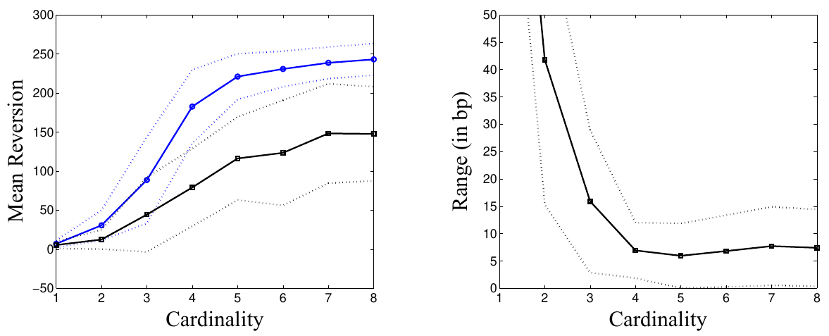
Look at the black squares against the blue circles, and then at the right-hand panel. Out-of-sample speed stays under in-sample speed and both rise with the number of names. The range, in basis points, falls. The paper does not print the coordinates, so the shape is the result: you buy out-of-sample speed by adding names, and you pay for it in how far the basket moves. The dashed lines are one standard deviation, and they are wide.
The dense canonical ranking, the thing the cap is refusing, is the table next to that idea. The fastest portfolio has mean reversion 238.11, volatility 0.07, and a p-value of 0.51. The other speeds are 0.58, 8.61, 16.48, 38.59, 84.55, 174.82, and 184.83. Every earlier p-value prints as 0.00. Volatilities run 0.21, 0.28, 0.34, 0.14, 0.10, 0.09, 0.07, 0.07. On a 252-day year, 174.82 is a half-life of 1.00 trading day and 184.83 is 0.95 trading days, both with the test the paper treats as significant. The 238.11 book is 0.73 trading days at the same volatility 0.07, and the p-value is 0.51. The paper attributes that insignificance to a one-day half-life on daily data. The seventh portfolio is also a one-day book and is marked significant. The table does not reconcile the sentence. The paper does not name the test. Keep the printed p-values, and do not promote 238.11 into a trade on the back of a point estimate the test does not believe.
The caption under that table says portfolio sizes from one to eight. The paragraph above it says eight canonical portfolios ranked by predictability, which on eight maturities are dense. The sparse weights are a different object. Their speeds are not these eight numbers. Read the columns as the ranked dense portfolios.
The dollar-cross sample does not repeat the swap slope. After the fourteen-name cut, out-of-sample speed was higher for the small baskets than for the full cluster, and the penalized Γ and A beat the raw estimates. Small baskets there also kept a wider range. Two markets, two shapes. The swap curve pays you speed for density and takes the range away. The cross cluster takes the speed away as well once the basket gets dense. Quoting one slope for both is how a cap chosen on swaps gets pasted onto a cluster of less liquid dollar crosses.
Charge the spread, then pick the smallest basket that still clears it
The convergence test is a different window from the range plot: parameters fit on 100 days, Sharpe ratio measured on the next 50.
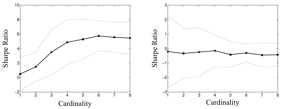
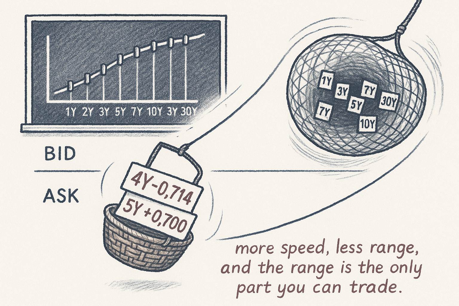
Look at the right-hand panel. A bid-ask spread of 1bp puts the out-of-sample Sharpe ratio on a flat line at or below zero. The left-hand panel, with the spread omitted, rises with cardinality on a grid that runs up to 10. The paper does not print the Sharpe values, only the figure, and the dashed bands are one standard deviation. The sentence in the text is the result: on these liquid swaps, 1bp neutralizes the inefficiency. The old article "Why Transaction Costs Should Be Added Before You Fall in Love" is the rule that panel is enforcing. The frictionless curve is the number a desk gets attached to. The 1bp curve is the one that has met a spread.
The appendix, before that bill, sizes a frictionless log-utility book. Wealth W and the basket price P have to be in the same units, because the wealth change includes N times dP. A swap rate in percent is not that price. You map x into a package of swaps with a DV01 you can warehouse, call the package's mark-to-market P, and only then is N a number of packages. The paper never prints that map. It is the missing input.
The stationary law the paper does print says the basket sits around its mean with variance σ squared over 2λ.
$$ s^{2} = \frac{\sigma^{2}}{2\lambda} $$
s is the stationary standard deviation. Hold s fixed and a faster λ comes with a larger σ. Those two enter the log-utility weight in opposite directions.
$$ \frac{N_t}{W_t} = \frac{\lambda(\bar{P} - P_t) - r P_t}{\sigma^{2}} $$
N over W is the number of packages per unit of wealth. The numerator is the reversion pull minus a financing term at rate r. The denominator is the diffusion variance. Set the mean to 0, ignore r for a moment, and substitute σ squared = 2λ s squared. The speed cancels. The weight equals minus P over 2 s squared.
Sketch, not a fit to the table: a one-trading-day half-life, so λ = 174.67 per year, a basket rich by P = 0.05, and s = 0.10, in whatever units you denominated the package. Then 0.05 / (2 × 0.01) = 2.50. You short 2.50 packages per unit of wealth. The financing term at r = 0.05 moves that by less than 0.01. Halve the stationary standard deviation and the weight quadruples, because s sits squared in the denominator. The quiet books are the ones that demand the leverage, and the quiet books are the ones whose range falls inside the spread. The 1bp panel is that arithmetic meeting a market.
I am against shipping the maximum-speed portfolio. On this paper's own table it is the insignificant one, and on this paper's own Sharpe figure a 1bp spread flattens every cardinality, including the dense end where the frictionless curve looks best. Run the greedy path forward and backward at each k. Plot out-of-sample speed and out-of-sample range in the same units as the spread you will pay, which is not a single number across the 2-year and the 30-year. Keep the smallest k whose range clears that spread by a margin you would warehouse, then charge the spread and read the Sharpe again. On the printed swap path that comparison starts at the 5-year, steps to the 4s5s slope, and steps again to the 3s4s5s butterfly. The pair is allowed to win. It wins when the butterfly's extra speed arrives with a range inside the bid and the ask. k chosen off the same plot is another degree of freedom, and the paper does not charge for the search over k, over ρ, or over the penalty that zeroed 20% of A.
KEY POINTS
- Minimize the lag's share of basket variance. In the two-name toy each name scores 0.50, the spread scores 0.20, and the sum scores 0.80.
- Cap the nonzeros and grow them greedily. The printed swap path starts at the 5-year with weight 1.000, then the 4-year at -0.714 against the 5-year at 0.700.
- Convert speed with the natural log of 2. A coefficient of 238.11 is 0.73 trading days on a 252-day year, and the printed p-value on that book is 0.51.
- Penalize the precision before you search. At a correlation of 0.90 and ρ = 0.10, the penalty at the unpenalized fit is 2.00 against a log-likelihood term of -0.34.
- Charge the spread before you pick k. A 1bp bid-ask spread flattens the out-of-sample Sharpe on these swaps; the frictionless curve is the one that omits it.
References
- Stat-Arb Is a Clustering Problem: Multi-View Spectral > Any Signal
- Why Transaction Costs Should Be Added Before You Fall in Love
- Identifying Small Mean Reverting Portfolios, Alexandre d'Aspremont
A note on AI. The ideas, research, analysis, and conclusions in this article are my own. I use AI tools to help with editing and wordsmithing, because English is not my first language, and I am not shy about that. AI-generated ideas and AI-assisted writing are not the same thing: the first is empty slop from a generic prompt, the second is a tool for communicating years of real research more clearly. Judge the work by its substance, not by whether software helped polish the prose.