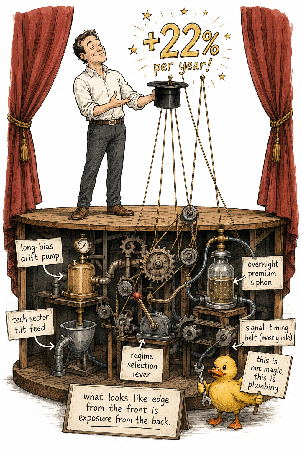
A backtest that shows a positive return proves nothing about predictive power. The returns might be drift collected by long bias, sector exposure collected by an implicit tilt, factor exposure collected by structural design, or any combination. The "edge" the trader sees on the equity curve might be zero once every exposure is accounted for.

The previous articles in this series covered the simplest version of this problem: a long-biased rule in an upward-drifting market collects free return from the drift. That is the visible trap. The hidden trap is more dangerous because it operates through exposures the trader did not explicitly choose and does not see in the rule's parameters. Sector tilt, factor tilt, regime tilt, and time-of-day tilt all produce returns that look identical to predictive edge on the surface and behave completely differently in live trading.

Most retail strategies that "work" in backtests and fail in live trading fail for exactly this reason. The backtest measured exposure. Live trading exposed the exposure.

The general exposure decomposition

Every backtest return can be decomposed into a sum of exposures times factor returns, plus a residual predictive contribution, plus noise.

Where β_i is the rule's average exposure to factor i during the test window, μ_i is the realized average return of factor i during the same window, α_predictive is the part of the return not explained by any factor exposure, and ε is residual noise.

The factors in the sum can be anything: market direction, momentum, value, size, quality, low volatility, specific sectors, specific countries, specific currencies, time of day, day of week, volatility regime, interest-rate regime. Any source of return that the rule is exposed to belongs in the sum.

A rule with edge has a non-zero α_predictive after every relevant β has been accounted for. A rule without edge has α_predictive ≈ 0; whatever the backtest showed came from the exposures. The job of evaluation is to estimate every β_i × μ_i correctly so that what is left in α is actually edge and not just an exposure the analyst forgot to subtract.

The forms of hidden bias

The visible bias (long/short percentage on a single market) is the easiest to detect and the easiest to fix. The hidden biases require explicit diagnostic work.

Sector or factor tilt. A rule that signals "long" on the QQQ from 2010 to 2021 is largely a long-tech bet. The rule's returns track the tech sector's outperformance over the period. The same rule on equal-weighted broad indices over the same period looks nothing like the QQQ version. The sector tilt was the source of the return, not the signal logic.

Time-of-day tilt. Most equity index returns historically accrue overnight. A rule that systematically holds positions across the close picks up the overnight risk premium regardless of any signal logic. Two rules that look identical except for whether they hold overnight or only intraday can have backtest Sharpe ratios that differ by a factor of two purely from this exposure.

Volatility regime tilt. A rule that is leveraged or fully invested only during low-volatility periods has selected the calmest portion of the historical sample. Low-vol periods historically correlate with positive drift. The rule's apparent risk-adjusted return is partially the regime selection, not the timing of any specific signal.

Country or currency tilt. A rule trading on multiple instruments that happens to be long EM during a strong EM decade is collecting the EM beta. The rule's returns generalize to nothing if EM weakens. Same logic applies to currencies, commodities, and any cross-sectional concentration.

Period selection tilt. Choosing the test window itself can hide bias. The 2009 to 2021 window has different statistical properties than any window containing 2000 to 2002 or 2008. A rule "tested over the past 12 years" on US equities is being evaluated in one specific drift regime. The choice of window is implicit bias and is often unreported.

Every one of these tilts shows up as positive backtest return without any signal-level edge. They are invisible in the rule's parameters and visible only after explicit factor accounting.

Worked example: the QQQ "trend follower"

A simple 50-day / 200-day moving average crossover rule on the QQQ ETF from 2010 to 2021. Long when the 50-day is above the 200-day, flat otherwise.

Headline backtest results:

• Annualized return: 22%
• Sharpe ratio: 1.4
• Long 88% of the time over the period
• Max drawdown: 17%

These numbers look like a discovery. They are not.

The decomposition:

• Buy-and-hold QQQ over 2010-2021: roughly 18% annualized. The rule was long 88% of the time, so its baseline drift collection is 0.88 × 18% ≈ 16%.
• The remaining 6% might be edge, or it might be additional exposure.
• The QQQ was a concentrated tech bet during this period. Equal-weighted S&P 500 returned roughly 14% annualized. The "tech sector tilt" beyond broad equity exposure contributed roughly 4 percentage points per year to QQQ. The rule's long QQQ exposure inherited this.
• The signal timing (the part that says "be long when 50 crosses above 200") contributed roughly 1 percentage point per year after both the drift and the tech tilt are removed.

The full decomposition:

• 16% from broad equity drift × rule's long exposure
• 5% from tech sector tilt × rule's long QQQ exposure
• 1% from actual signal timing (the edge)
• 22% headline

The rule is 95% equity beta and tech sector tilt. The signal contribution is small enough that transaction costs would consume most of it. In live trading from 2022 onward, the rule lost money. The tech tilt that contributed 5% per year on the way up subtracted on the way down. The "edge" was beta in disguise.

Diagnostic tests for hidden bias

Six tests, in increasing order of sophistication, that separate bias from edge.

1. Detrended re-run. Subtract the market's mean daily return from each day's return. Re-run the rule on the detrended series. A bias-driven rule's return collapses toward zero. An edge-driven rule keeps most of its performance.

2. Signal permutation. Keep the actual market returns intact. Randomly permute the rule's signal timestamps 5000 times. Compute the rule's return on each permutation. The distribution of permuted returns is what the rule earns from its exposures alone, with no timing edge. If the actual rule return sits inside this distribution, the rule has no timing edge. If it sits outside the tail, there is signal.

3. Bias-matched random rule. Generate 5000 random rules with the same long/short proportions as the actual rule. Each random rule has no signal logic. Compute the mean return of each. The actual rule's return minus the mean of the matched-random distribution is the predictive contribution. If this gap is small relative to the noise in the matched-random distribution, the rule is bias.

4. Regime split. Partition the test window into bull, bear, and sideways sub-periods using a regime classifier (e.g., 200-day moving average sign, trailing 12-month return sign, or volatility regime). Compute the rule's return in each sub-period. A pure-bias rule shows extreme regime dependence (great in bulls, terrible in bears). An edge-driven rule shows moderate regime dependence and positive results across regimes.

5. Factor regression. Regress the strategy's daily returns on a multifactor model (market, size, value, momentum, quality, plus relevant sector or currency factors). The intercept of the regression is the alpha after factor exposures. The R² is how much of the strategy's return the factors explain. A strategy with R² of 0.9 against a standard factor model has 10% of its return left over as alpha. That 10% is the candidate edge; the rest is factor exposure that could be obtained more cheaply via ETFs.

6. Instrument swap. Apply the same rule with the same parameters to a different but related instrument (e.g., QQQ rule applied to SPY, or SPX rule applied to FTSE, or US trend rule applied to JP trend). Edge tends to generalize across closely related instruments. Pure bias does not, because the bias was specific to the drift of the original instrument during the original window.

A strategy that passes all six tests has earned the benefit of the doubt. A strategy that fails any of them is bias dressed as edge.

Visualizing the iceberg

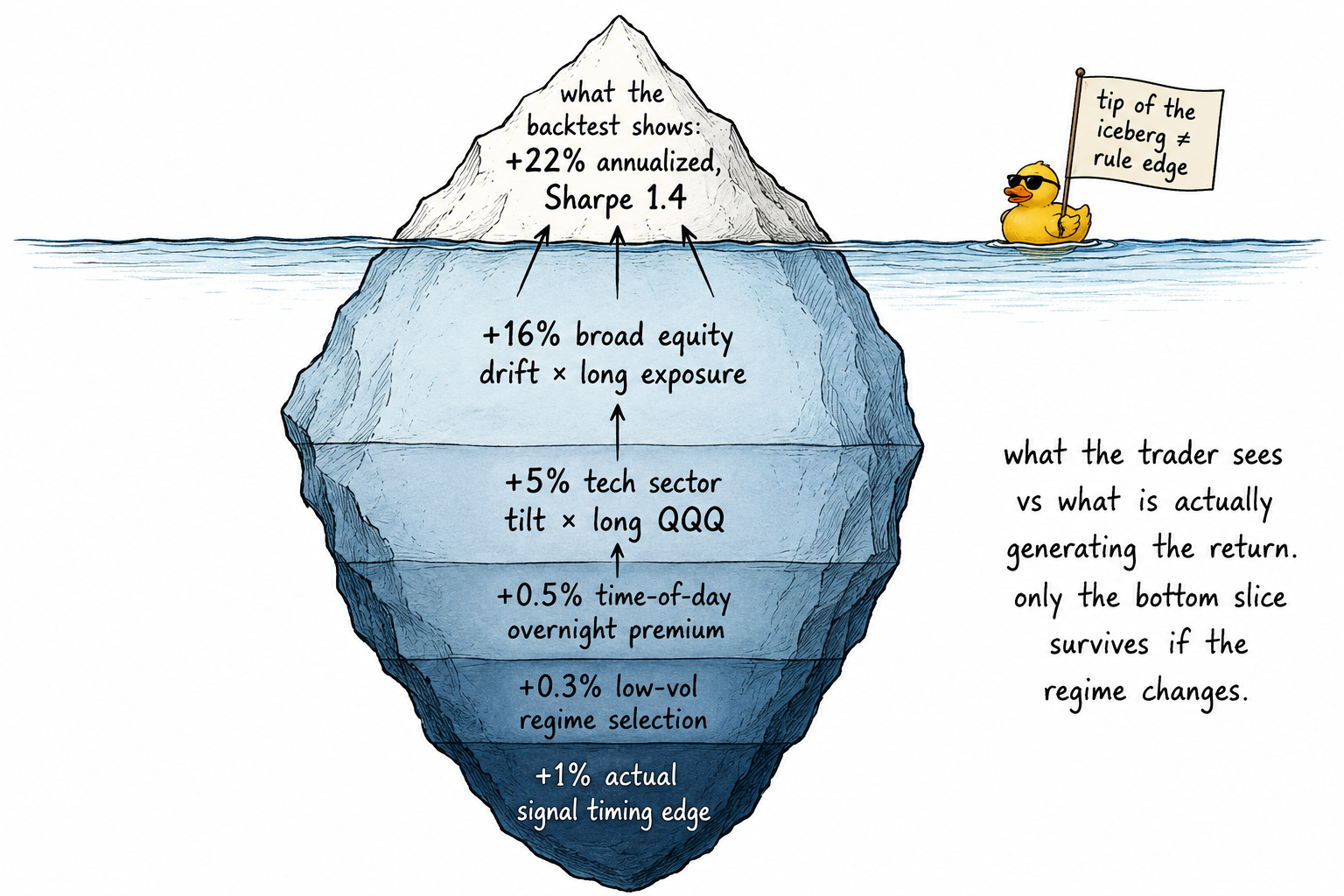
The picture is the trap. The trader sees the tip. The actual return generation is below the waterline. When the regime changes, the layers below the waterline change sign and the tip melts.

The non-stationarity twist

Hidden bias becomes more dangerous when the regime shifts.

A 90% long bias on US equities from 2009 to 2021 collected approximately 10% per year of free drift. The same 90% long bias from 2000 to 2002 lost that drift back, and then some. A rule that was implicitly betting on tech sector outperformance from 2010 to 2021 was implicitly betting on tech sector underperformance whenever that tilt reversed.

Bias is a directional bet whose value depends on the regime. In a backtest restricted to one regime, the bet looks like a free return. In live trading across regime shifts, the same bet is a leveraged exposure to whichever direction the regime takes.

This is the mechanism by which "great backtests" become "live losses." The hidden bias was net positive in the historical sample and turns net negative in the next sample. The signal logic, which was never the source of the return, has nothing to contribute when the bias contribution goes negative.

Why the trap stays hidden

The trap stays hidden because every default reporting practice favors the headline number.

The annualized return is reported. The Sharpe ratio against zero is reported. The equity curve goes up. The drawdown looks manageable. None of these surface the underlying decomposition.

The factor regression, the regime split, the bias-matched comparison, and the signal permutation are all extra work. Most strategy reports omit them. The trader who runs them sees fewer publishable strategies, makes fewer overconfident claims, and has fewer live failures. The trader who does not run them ships more strategies, sounds more confident, and discovers the decomposition in production at considerable cost.

The path of least cognitive resistance is to accept the headline. The path of least financial damage is to refuse to.

What this changes operationally

Three changes.

Every strategy report should include the bias decomposition. Headline return, exposure contributions, residual alpha. Without this breakdown, the headline number is incomplete information.

Every strategy should pass at least three of the six diagnostic tests before being approved for live trading. Different rules require different diagnostics: a long-biased equity timing rule needs the detrended re-run and the regime split; a multi-asset rule needs the factor regression and the instrument swap; a timing rule on a single asset needs the signal permutation and the matched-random comparison.

Treat positive backtest returns as a starting point for investigation, not as proof of anything. The default assumption is that the return came from bias. The burden of proof is on the trader to show that residual alpha exists after every exposure is accounted for.

KEY POINTS

• A backtest with positive return proves nothing about predictive power. The return decomposes into a sum of exposure × factor contributions plus a residual α_predictive plus noise.
• Hidden biases beyond visible long/short percentage include sector tilt, time-of-day tilt, volatility regime tilt, country/currency tilt, and test-window selection tilt. Each generates positive return without any signal-level edge.
• The QQQ 50/200 trend rule from 2010 to 2021 returned 22% headline. Decomposition: 16% from broad equity drift × long exposure, 5% from tech sector tilt, 1% from actual signal timing. The signal contributed almost nothing once factor exposures were stripped out.
• Six diagnostic tests separate bias from edge: detrended re-run, signal permutation, bias-matched random rule, regime split, factor regression, instrument swap. A strategy that passes all six has earned the benefit of the doubt.
• Bias is a directional bet whose value depends on the regime. The same long bias that collected 10% per year of drift in a bull regime can lose more than that in a bear regime. Backtests over single regimes hide this risk.
• The trap stays hidden because the default reporting (headline return, Sharpe vs zero, equity curve) does not surface the decomposition. The factor regression, regime split, and permutation test are extra work that most strategy reports skip.
• Treat positive backtest returns as a starting point for investigation, not as proof. The default assumption is that the return came from bias. The burden of proof is on the trader to demonstrate residual alpha after every exposure is accounted for.