1.28 Five Definitions of Fair Value, and the Trade Each One Implies

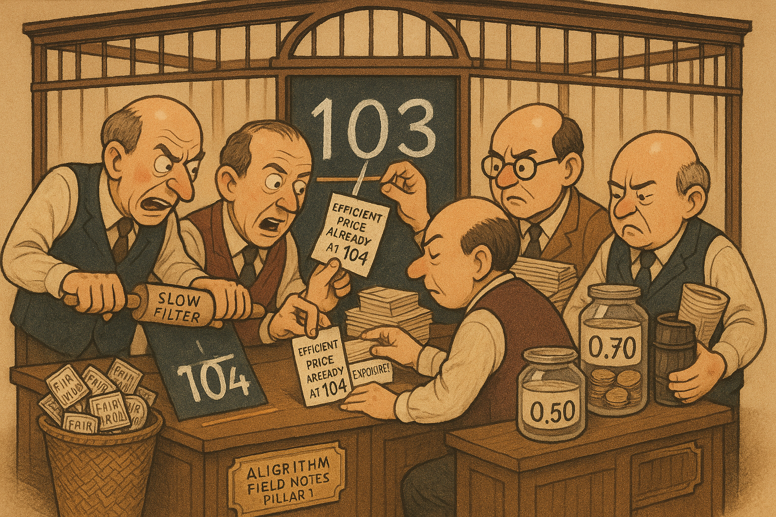
Fair value is the number you subtract before you put the trade on, and that subtraction is the strategy. On the Hyperliquid BTC-USD perpetual in September 2025, a post-only buy, refused if it would cross the spread, never rests in the book, and the mid, the average of the best bid and the best ask, still returns 0.31 basis points over the next ten seconds in the buy's direction. A low-pass filter of that same print fades the excursion off its slow curve. A factor model skips the print and assigns an expected excess return from exposures. An event contract priced at 0.70 is a probability whose expected change, under the pricing measure, is zero. A crude book judges West Texas Intermediate only against Brent and Dubai, and a level that is cheap on one of these subtractions can be rich on another.

Fade the print toward the slow curve

The old article "Fair Value as an Adaptive Low-Pass Filter: LAFO for Mean Reversion" treats fair value as the output of a low-pass filter. LAFO, the local average filtering objective, does not score the filter on every tick. It scores the average residual inside a window of length K.

$$ \mathcal{L}_{\text{LAFO}}(\hat{y}) = \frac{1}{T} \lVert A(y - \hat{y}) \rVert_2^2 $$

A is the operator that replaces each residual with the average residual over the window that ends on that bar. T is the length of the sample. You are minimizing the squared length of those windowed residuals. Set K to 1 and A is the identity, so LAFO is ordinary mean squared error and the filter chases every wiggle. Set K to T and the objective only sees the average residual of the whole sample, so the best fit is the global mean. Take residuals of +3, 0, and −3. At K equal to 1 the loss is the average of 9, 0, and 9, which is 6. At K equal to T the residuals sum to 0, the windowed residual is 0, and the loss is 0. Same three numbers, opposite verdict. The K you trade sits between those poles. A penalty on the changes in the fitted curve, total variation, an l1 penalty on slope changes, or an l2 penalty on steps, then decides whether that curve jumps in flat steps, bends in straight segments, or drifts smoothly. The old article draws the three.

The trade is the fade of the relative gap, with a deadband that keeps the position flat inside the noise.

$$ \delta_t = \frac{y_t - \hat{y}_t}{\hat{y}_t}, \qquad w_t = -\operatorname{sgn}(\delta_t)\,\min\{1,\ \alpha \max(0,\ |\delta_t| - \tau)\} \quad \text{when } |\delta_t| \ge \tau $$

Delta is the percentage gap between the print and the filter. Tau is the band inside which the position is zero. Alpha scales the excess gap, and the position is capped at 1. The minus sign means you short a print that sits above the curve. The old article uses the demo's settings, tau of 0.0005 and alpha of 200. Spot 5005 against a filter of 5000 is a gap of 5 over 5000, which is 0.001. That clears the band by 0.0005. Alpha times 0.0005 is 0.10. You are short a tenth of full size. Spot 5000.5 gives a gap of 0.0001, inside the band, and you are flat. The bet is that the wiggle dies inside the window and the slow curve was the right subtraction. A regime break inside that window is the bet losing: you are short a curve that has already moved.

The fair number is an expected return

The old article "What a Factor Actually Is: α + βλ, and Why the Market Is Factor #1" hangs the cross-section on one line. Chuan Shi's lecture writes the same line as the model of the mean. Pricing theory arrives at it from a stochastic discount factor, the random variable that turns a future payoff into a present price. The lecture does not derive that factor. It starts from the line.

$$ \mathbb{E}[R_i^e] = \alpha_i + \beta_i^{\top} \lambda $$

The left side is the expected excess return of asset i, its average return above the risk-free rate. Lambda is the vector of factor risk premiums. Beta is the vector of that asset's exposures. Beta-transpose lambda is the return the model pays the asset for carrying those exposures. Alpha is the pricing error, the leftover. The filter section uses the same letter for a position scale; here it is an expected return. The loadings below are chosen so the arithmetic is visible. The lecture does not print them. Load 1.2 on the market, 0.4 on value, and −0.3 on momentum, with annual premiums of 6, 3, and 4 percent. The model return is 1.2 times 6, plus 0.4 times 3, minus 0.3 times 4, which is 7.2 plus 1.2 minus 1.2, so 7.20 percent. An asset that averaged 9 percent has an alpha of 1.80 percent. An asset that averaged 7.20 percent has an alpha of zero, and the price level never entered the calculation.

A nonzero alpha leaves two trades. The equation is silent on which. If you will say the factor list is complete, trade the residual: long the name and short the factor book. If the 1.80 percent is a premium the list forgot, add the factor and leave the residual alone. Shi states Fama's joint hypothesis in those terms: a test of efficiency is also a choice of model. The lecture states that expected excess returns do not line up with market betas, which is why the vector replaced the scalar. The old article's point stands next to that. Remove the market exposure first, because it explains more return variance than the next characteristic you test.

Leave the probability where it printed

The old article "A Black-Scholes for Beliefs: Logit Jump-Diffusion and Tradable Belief-Vol" maps an event contract through log-odds so the state variable is unbounded. Dalen, writing with the Daedalus Research Team, sets the traded price p between 0 and 1 equal to a sigmoid of a latent logit x. The contract pays one dollar if the event happens and zero otherwise. Under the pricing measure, p is a martingale, so its drift is zero.

$$ x = \log \frac{p}{1-p}, \qquad p = \frac{1}{1+e^{-x}} $$

A price of 0.70 is a logit of the log of 7/3, which is 0.847. A price of 0.50 is a logit of zero. The map is one-to-one.

The drift of x is pinned so that the expected change in p is zero. Dalen's equation (3) subtracts a jump compensator as well as the diffusion term. Set the jump measure to zero and the drift collapses.

$$ \mu = -\frac{1}{2}(1-2p)\,\sigma_b^2 $$

Sigma-b is belief volatility, the scale of the Brownian piece in the logit. The slope of the sigmoid is p times one minus p. The curvature is that slope times one minus two-p. For the diffusion, the expected change in p over a short step dt is the slope times mu times dt, plus one-half the curvature times sigma-b squared times dt. Those two pieces are built to cancel. At p equal to 0.70 and sigma-b equal to 1, one minus two-p is −0.4, so mu is 0.20. The slope is 0.21 and the curvature is −0.084. Over dt of 0.01 the drift piece moves p by 0.21 times 0.20 times 0.01, which is +0.00042. The curvature piece moves p by one-half times −0.084 times 0.01, which is −0.00042. The expected change in the contract is zero. The logit drifts up because the sigmoid is concave above one-half, and that concavity would otherwise pull p down. The event did not become likelier.

The trade this definition allows is in belief volatility, jump intensity, and cross-event dependence. The old article builds the variance swap on the logit. Fading 0.70 toward 0.50 is a different bet, and this kernel says that bet has no edge under the pricing measure. Under the physical measure a risk premium can exist. Dalen does not estimate one.

Cheap means cheap against the basket

The old article "Mean-Reverting Stat-Arb in Crude Oil: WTI vs Brent/Dubai" builds Fanelli's book. Fair value of West Texas Intermediate is the fitted value of a cointegrating regression on Brent and Dubai. Cointegration here means each crude price can wander, while a fixed linear combination of the three does not. The mispricing is the residual.

$$ M_t = Z_t - \big(c + h^{1} v^{1}_t + h^{2} v^{2}_t\big) $$

Z is the WTI futures price. The first futures price is Brent, the second is Dubai, c is the intercept, and the h coefficients are the basket weights. You are long one WTI, short h-one Brent, and short h-two Dubai. A negative h-two is a long Dubai leg. On the full weekly sample, 461 observations from 25 October 2000 to 19 October 2009, the regression prints c of 1.61763, h-one of 1.19378, and h-two of −0.21702, with an R-squared of 0.995. Put all three crudes at 50 dollars. The fitted WTI is 1.61763 plus 1.19378 times 50 plus −0.21702 times 50, which is 1.61763 plus 59.689 minus 10.851, which is 50.46. WTI at 50 is cheap by 0.46 dollars against that basket.

The note under her weekly table writes a minus in front of each weight. The same coefficients with that minus fit WTI at 1.61763 minus 59.689 minus −10.851, which is −47.22. A fitted price of −47 dollars in a 50 dollar market is the regression running backward. Her daily section writes the plus form, and the portfolio prose is long WTI against the basket, which is the plus form again. Use the plus form. The minus in the weekly note may be a source error. The old article flagged it.

The position fades last week's residual. The exponent k is Fanelli's sensitivity. The LAFO window is a different K.

$$ S_t^{k} = -\operatorname{sign}(M_{t-1})\,|M_{t-1}|^{k} $$

The sign is the sign of last week's residual, and the absolute residual is raised to k before the leading minus flips the side. Sell the book when this signal is negative. A residual of +4 dollars means rich WTI. At k equal to 0 the position is −1, a one-unit step. At k equal to 1 the position is −4. Same side, four times the size. The exponent scales the position with the gap. On the 50 dollar case the residual is −0.46, k equal to 1 is a long of 0.46, and k equal to 0 is a long of one full unit. She then damps the position with a moving average and a smoother. The old article shows that the weekly formula, the daily formula, and the figure caption are three different recursions, so if you code this, pick one of them on purpose.

The weights break. A Quandt likelihood ratio, the maximum of the break tests over the middle 70 percent of the sample, prints 61.27. The paper calls that number a critical value. It is the test statistic, and on their reporting it rejects stable weights at the 1 percent level. She dates the break at 14 February 2005. Before it, Brent's weight is 0.976 and Dubai's is 0.185, so both are shorts against long WTI. After it, through the end of 2007, Brent's weight is 1.316 and Dubai's is −0.317. The Dubai leg has moved to the long side. Keep the pre-break hedge through that date and you are short a leg the regression now wants long. The bet is that the residual mean-reverts and the weights you estimated are still the relation. A break, or a residual with a unit root, is the bet dying.

The efficient price has already moved

Dalen writes the print as a noisy observation of a latent logit, and calls the fit of that noise Hasbrouck-style. This is the fifth subtraction. The efficient price is the latent level. The print is that level plus a transitory error. You fade the error. You do not fade the latent level toward a slower curve.

$$ y_t = x_t + \eta_t $$

Y is the logit of a trade-weighted mid. X is the latent logit, the efficient price in logit units. Eta is microstructure noise. Dalen lets the noise variance depend on the spread, depth, trade rate, and aggressor imbalance. The logits 0.85 and 1.05 are chosen so the gap is easy to see. A latent logit of 0.85 is a probability of 0.7006. An observed logit of 1.05 is a probability of 0.7408. The noise is 0.0402 on a one-dollar contract, about four cents. The efficient-price trade sells the rich print back toward 0.7006. It does not sell 0.7006 toward 0.50. That second sale is the martingale section's forbidden fade, and it is also what a slow filter does when its curve lags the latent level.

Albers, Cucuringu, Howison, and Shestopaloff supply the tape version of the same split, on a book where the latent level is not observed. Their object is the post-submission price return, the mid return in basis points over the next ten seconds, regressed on a signed refusal.

$$ R_t = \beta_0 + \beta_1 \mathbf{1}_t^{\text{rej}} + \epsilon_t $$

The indicator is +1 for a refused buy and −1 for a refused sell. The intercept is −0.1178 and the slope is 0.4242, both with a standard error of 0.0003, on the September 2025 Hyperliquid sample. A refused buy forecasts −0.1178 plus 0.4242, which is 0.3064 basis points. A refused sell forecasts −0.1178 minus 0.4242, which is −0.5420 basis points. Add the intercept before you quote the slope as the forecast. The R-squared is 0.022. Add the refused-volume imbalance inside the last 100 post-only submissions, accepted or refused: refused buy volume minus refused sell volume, over the sum. The single-order slope falls from 0.4242 to 0.1354, and the flow imbalance takes a coefficient of 0.5415. The one order was a symptom of a crowd leaning the same way. The R-squared rises to 0.033.

Their comparative regression, the one they label (5), puts the visible top-of-book imbalance, the standardized spread, the refused-flow imbalance, and the opened-order imbalance in one line. The coefficients are 0.6224, 0.0305, 0.1674, and 0.0705, with an intercept of −0.1366 and an R-squared of 0.045. The refused flow still loads after the visible book, at more than twice the opened-order imbalance (0.1674 over 0.0705 is 2.37). Set every imbalance to +1 and the spread to 0, which is the daily mean of a series they standardize every day. The fitted return is −0.1366 plus 0.6224 plus 0.1674 plus 0.0705, which is 0.7237 basis points. The paper calls this corner "at most a few tenths of a basis point." The printed coefficients sum to 0.72 to two decimals. Keep 0.72, and treat the phrase as looser than the table.

The taker fee on that venue runs from 1.44 to 2.7 basis points. A forecast of 0.31, or of 0.72 with every imbalance pinned at the extreme, does not pay the cheapest fee. The directional hit rate is still high: a refusal matches the next price change 72.3 percent of the time, and the median wait to that change is about two seconds. There are about 60,310 such refusals a minute, 86 percent of order submissions, on the order of 3.3 billion dollars of notional a minute at the average refused size of 54,693 dollars. The trade the efficient-price definition implies, on this tape, is to stand aside as a taker. The print is late relative to a latent level you cannot see, the lateness is a fraction of the fee, and paying the fee to harvest it is the losing side. Someone running the queue-priority strategy that generates the refusals is trying to be first at the new best price, which is a different trade from the ten-second return.

The grey bands are opposite sides

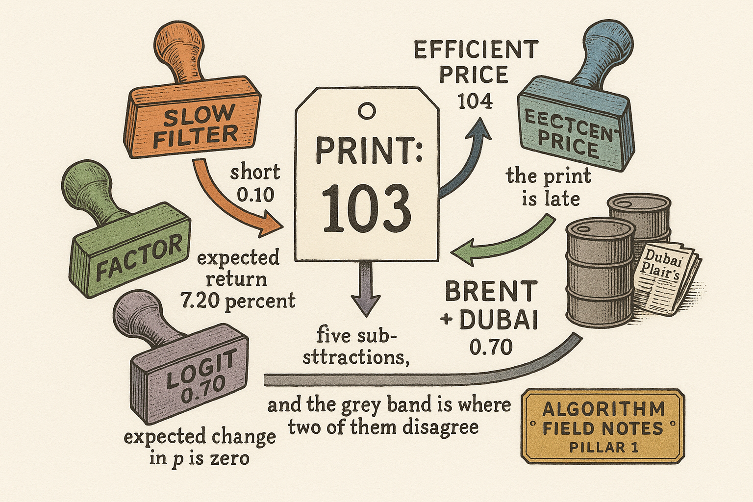
Look at the grey bands. The black print sits above the orange slow filter and below the blue efficient price, so the fade is short and the catch-up is long.

The path is constructed. Bar 80 is one of the grey bars: the print is 103, the filter is 102.025, and the efficient price is 104. A filter rule shorts the print toward 102.025. An efficient-price rule buys it toward 104. Same print, opposite side, and the only thing that changed is which subtraction you called fair.

On the papers' own scales that conflict is a short of 0.10, a refused-buy forecast of 0.31 basis points, and a taker fee that starts at 1.44 basis points. The rest of the grid is the same kind of check: the value ETFs in Shi's lecture, from 30 April 2013 to 31 March 2020, returned 4.30 percent for Vanguard Value and 0.41 percent for the Invesco pure-value fund against 7.35 percent for the S&P 500; Fanelli's out-of-sample years printed 4.97, 30.26, and 4.90 percent, so 2009 does the lifting; Dalen's Table 1 gives the logit jump-diffusion an MSE of 70.28 against 77.41 for a constant-volatility logit, while the random-walk row wins mean absolute error at 1.16 against 1.59 and the ARMA-GARCH row wins QLIKE, the volatility score that punishes an under-prediction, at 0.80 against 1.46, and the paper's text still calls the jump-diffusion best on mean absolute error; the Wright-Fisher row prints an MSE of 1.71 times 10 to the 17 and the ARMA-GARCH row prints 1.07 times 10 to the 19 once those baselines are mapped into logits, which is a numerical blow-up; the old article records an in-sample 2-minute Sharpe of 11.05 for a two-layer net and −18.27 for a 10-bar exponential moving average, on two months, with the authors calling the exercise a demo.

Write down what would prove the subtraction wrong

Name the object before you size anything. A slow filter is falsified when the gap does not close inside the window on a later sample. The old article records that the demo never makes that choice: the window, the penalty, the band, and the scale sit on the same two months as the Sharpe, and the authors leave the out-of-sample test to another paper. Until you pick K on data you have not traded, the short of 0.10 is a description of a fit.

A factor alpha is falsified when it disappears once the missing factor is in the list, or when it fails after cost on a later cross-section. Those value ETFs lost to the S&P over that seven-year window while still carrying the value label. Harvesting beta-transpose lambda can be the wrong side for years, and the equation will look the same on the day you put the trade on.

A logit martingale is falsified, as a pricing statement, if you can harvest a drift in p after the spread. Dalen's forecast test does not answer that. Section 6.2 says the series are 20 Polymarket events with noise added. The caption of Table 1 says a synthetic path. Score whichever sample you believe. The two sentences describe different samples. Dalen does not estimate a physical-measure premium.

An oil residual is falsified when the break test rejects and you keep the old weights, or when Dubai cannot be hit. Dubai is a Platt's assessment. The old article already treats that leg as a quote you cannot lift. Fanelli charges 0.25 percent on the change in position. A weight that flips sign on 14 February 2005 will charge you that cost on the day you admit the flip, and it will charge you the residual if you do not.

A refused-order coefficient is falsified as a taker trade by the fee, and as a real-time signal by the feed. The node that sees the refusals arrives too late for the ten-second horizon. The paper says so. What survives is a narrower claim: a flow with no footprint in the book still lines up with the next mid, the visible imbalance does not swallow the coefficient, and the size of the lineup is smaller than the toll for crossing.

I am against stacking the five gaps into one feature and letting a fit pick the sign. The sign is the hypothesis. Write the subtraction, the horizon, the cost, and the observation that would kill it. Then you have a strategy a later sample can refuse.

KEY POINTS

• Fade the slow curve with a deadband. Spot at 5005 against a filter at 5000, with the band at 0.0005 and the scale at 200, is a short of 0.10.
• Do not cross the spread on a refused post-only buy. The ten-second mid forecast on Hyperliquid is 0.31 basis points.
• Treat a leftover alpha as a trade only if you will say the factor list is complete. On the worked loadings that leftover is 1.80 percent a year.
• Leave an event contract at 0.70 where it printed. With no jumps and belief volatility of 1, the log-odds drift that keeps the probability a martingale is 0.20.
• Re-fit the crude basket when a weight changes sign. Dubai's cointegrating weight goes from 0.185 to −0.317 on 14 February 2005.

References

• Fair Value as an Adaptive Low-Pass Filter: LAFO for Mean Reversion
• What a Factor Actually Is: α + βλ, and Why the Market Is Factor #1
• A Black-Scholes for Beliefs: Logit Jump-Diffusion and Tradable Belief-Vol
• Mean-Reverting Stat-Arb in Crude Oil: WTI vs Brent/Dubai
• The Price Impact of Nothing: Rejected Orders as Predictors of Future Returns*
• Intro to Factor Investing
• Toward Black–Scholes for Prediction Markets: A Unified Kernel and Market-Maker’s Handbook
• Mean-Reverting Statistical Arbitrage Strategies in Crude Oil Markets

A note on AI. The ideas, research, analysis, and conclusions in this article are my own. I use AI tools to help with editing and wordsmithing, because English is not my first language, and I am not shy about that. AI-generated ideas and AI-assisted writing are not the same thing: the first is empty slop from a generic prompt, the second is a tool for communicating years of real research more clearly. Judge the work by its substance, not by whether software helped polish the prose.