2.39 Modeling Price as a Sine Wave: Instantaneous Frequency from 4 Points
Model price as one local sine and solve its frequency from four bars: difference out the offset, ratio out the amplitude, read cos(omega). Low lag, high variance, and it lies when no cycle exists.
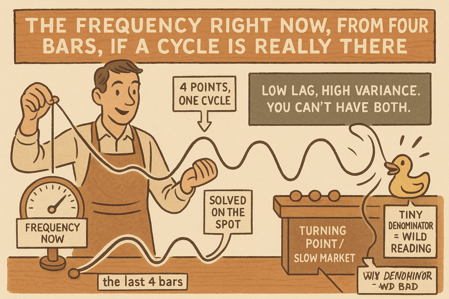
The old article "Dominant Cycle Estimation Without Astrology" measured the dominant cycle with autocorrelation and periodograms, methods that carry 12 to 32 bars of lag because they need a long window to resolve a frequency. This article shows the opposite extreme: assume the price is locally one sine wave and you can solve for its frequency from just four bars, with almost no lag. The math is exact and the appeal is obvious. The danger is equally obvious once you remember the old article "Why Market Cycles Are Evanescent": a four-bar frequency estimate is only as real as the assumption that four bars actually contain a clean cycle, and most of the time they do not.
One dominant cycle, four unknowns
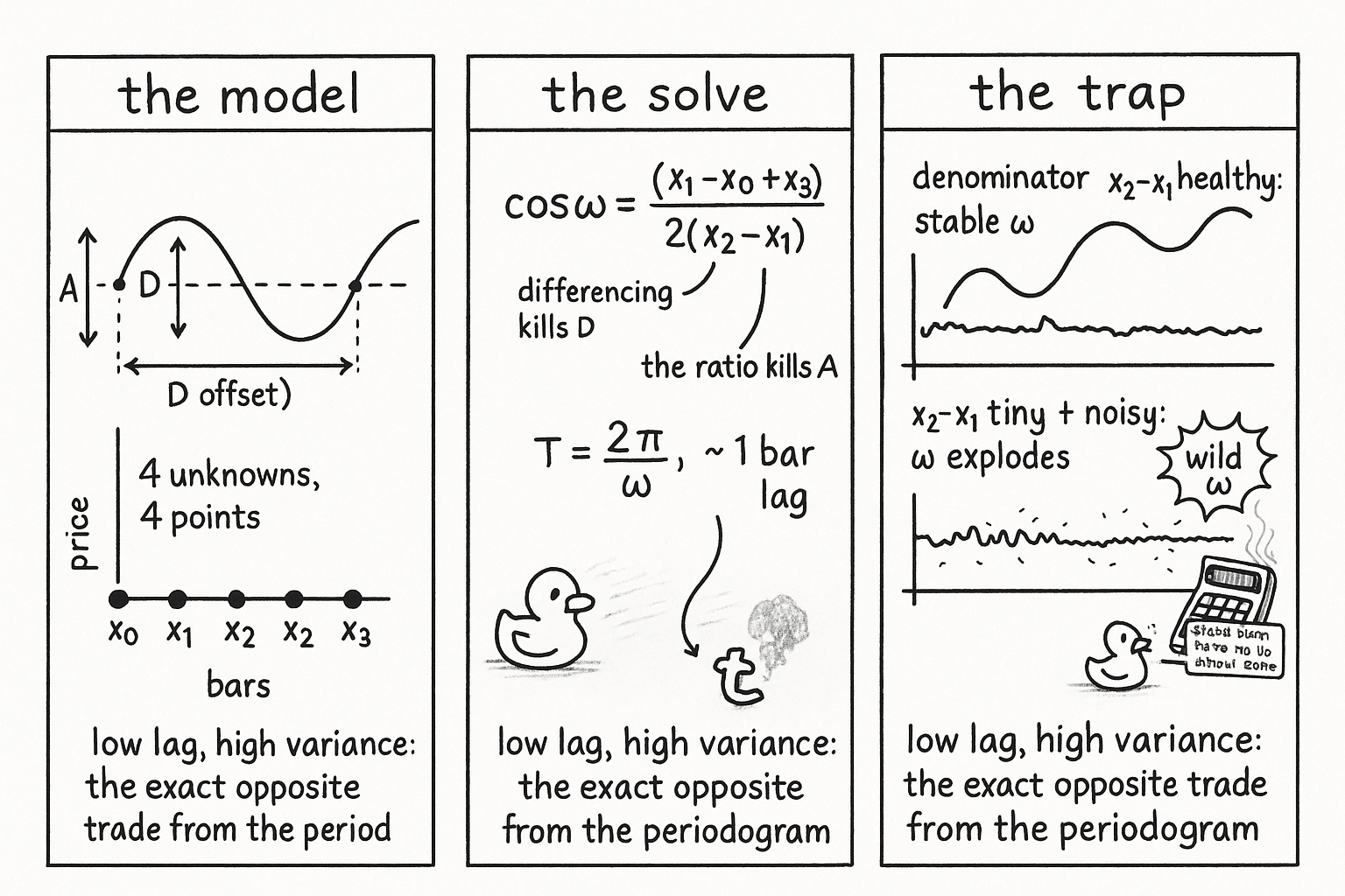
The model is the simplest thing that can oscillate: a single sine wave sitting on a constant level.
$$ x_t = A \sin(\omega t + \varphi) + D $$
Four unknowns live here: the amplitude A, the frequency omega, the phase phi, and the DC offset D. Four unknowns need four equations, which means four data points, the last four bars. Solve the system and you get omega, and from omega the period falls out as two pi over omega. The frequency you recover this way is the instantaneous frequency: how fast the market is oscillating right now, measured locally, not averaged over a long window. That locality is the whole selling point, because a long-window estimate tells you what the cycle was, while this tells you what it is, if the assumption holds.
The classical route to instantaneous frequency is the Hilbert transform, which builds in-phase and quadrature components and reads the rate of phase change. It works but it smooths, so it carries delay. The four-point solve is the low-lag alternative.
Difference away the offset, and the frequency falls out
The clean way to solve the system is to kill the unknowns you do not want. The DC offset D is a nuisance, so difference the series: consecutive differences of a sine are themselves a sine with the same frequency and no constant term. A pure sinusoid obeys a three-term recurrence, each sample is a fixed multiple of the average of its two neighbors, and that multiple is the cosine of the frequency. Apply it to the differenced series and the frequency comes out in closed form from four raw bars.
$$ \cos\omega = \frac{(x_1 - x_0) + (x_3 - x_2)}{2\,(x_2 - x_1)}, \qquad T = \frac{2\pi}{\omega} $$
The numerator and denominator are built from the three first-differences of the four bars, which is why D drops out: differencing removed it, and the ratio removed the amplitude A. What survives is the frequency alone. Take the arccosine, convert to a period, and you have measured the local cycle from four bars with effectively one bar of lag. No autocorrelation window, no periodogram, no 30-bar warmup.
Why this is fragile, and how it fails
The elegance hides a brutal sensitivity, and it lives in the denominator. The divisor is x2 minus x1, a single one-bar difference. When price is near a turning point or moving slowly, that difference is tiny, and dividing by a tiny noisy number blows the estimate up: the recovered frequency swings wildly from bar to bar on what is mostly measurement noise. A four-point estimator has no averaging to lean on, so every tick of noise lands directly in omega. The methods from the old dominant-cycle article paid 12 to 32 bars of lag precisely to buy the stability that this one throws away.
So the four-point frequency is high-variance by construction, the mirror image of the low-variance, high-lag periodogram. That is not a flaw to patch, it is the trade. The honest deployment follows from it. Smooth the raw four-point estimate before you trust it, which gives back some of the lag you saved but tames the explosions. Gate it on amplitude: when A is small there is no cycle to measure and the number is garbage, so suppress it. And hold the deeper skepticism from the old article "Why Market Cycles Are Evanescent": the model assumes one dominant clean cycle, and when the market is trending or thrashing there is no such cycle, so a confident four-bar frequency is then a precise measurement of something that is not there. Use it where a cycle demonstrably exists, distrust it everywhere else.
KEY POINTS
- Model price locally as one sine on a constant level, with four unknowns (amplitude, frequency, phase, offset). Four unknowns need four bars, so you can solve for the frequency from the last four points.
- The result is instantaneous frequency: the cycle speed right now, measured locally, versus the old article "Dominant Cycle Estimation Without Astrology" which averages over a long, lagging window.
- Difference the series to kill the offset D and form a ratio to kill the amplitude A; a sinusoid's three-term recurrence then gives cos(omega) from the four bars, and the period is two pi over omega, with about one bar of lag.
- The denominator is a single one-bar difference. Near turns or in slow markets it goes tiny and noisy, so the frequency estimate explodes. The estimator is high-variance by construction, the exact opposite trade from the high-lag periodogram.
- Deploy it by smoothing the raw estimate (giving back some lag for stability) and gating on amplitude, since a small A means no cycle and a garbage number.
- The old article "Why Market Cycles Are Evanescent" still binds: the one-clean-cycle assumption fails in trends and chop, where a confident four-bar frequency precisely measures a cycle that is not there.
References
- Statistically Sound Indicators for Financial Market Prediction - Timothy Masters (Amazon)
- Cycle Analytics for Traders - John Ehlers (Amazon)
- Instantaneous phase and frequency (Wikipedia)
- Hilbert transform and the analytic signal (Wikipedia)
- Frequency estimation from three samples of a sinusoid (recurrence relation, DSP StackExchange)
- MESA Software Technical Papers: instantaneous frequency and the Hilbert transform (John Ehlers)