7.2 Dynamic Time Warping for Time-Series Alignment
Fixed-lag cross-correlation assumes the delay between two markets never moves. It does. Dynamic time warping aligns two series with a stretchable path, scoring shape similarity and recovering a lead-lag that varies through time.
The lagged cross-correlation has a hidden assumption baked in. The old article "Lead-Lag Relationships in Global Markets" measured a lead by sliding one series against another by a fixed number of bars and finding the lag that lined them up best. That works when the delay between two markets is constant. It is not constant. The leader sometimes races ahead by two seconds, sometimes by ten, and a single fixed shift smears all of that into one blurry average. Dynamic time warping fixes the rigidity: instead of one shift for the whole series, it lets the alignment stretch and compress along the way so each point in A is matched to the point in B it actually corresponds to.
The old article "Crypto Cross-Exchange Lead-Lag Study" built the fixed-lag version on crypto venues. This is the tool you reach for when that fixed lag stops fitting because the delay itself is moving.
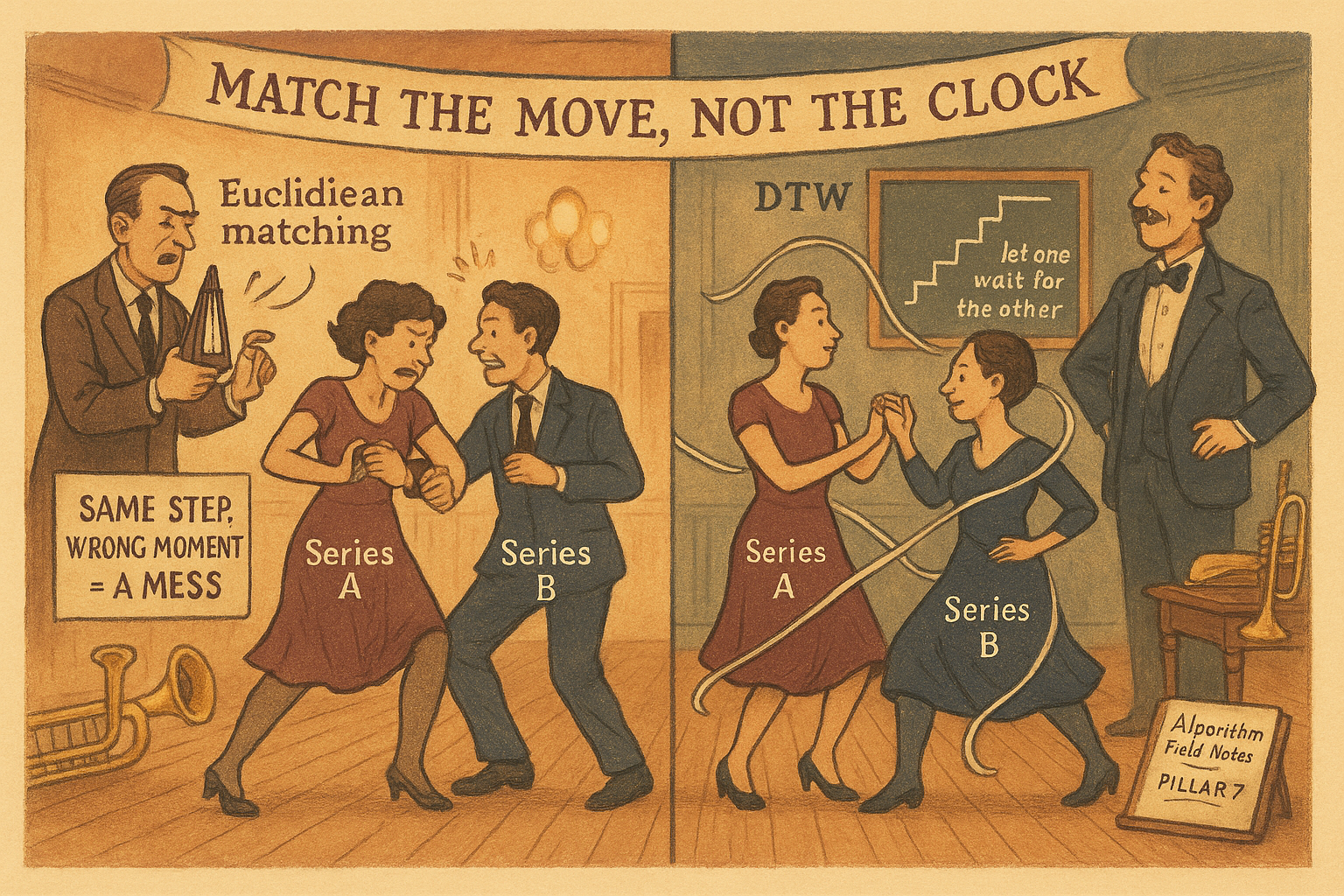
Euclidean matching is point-for-point and brittle
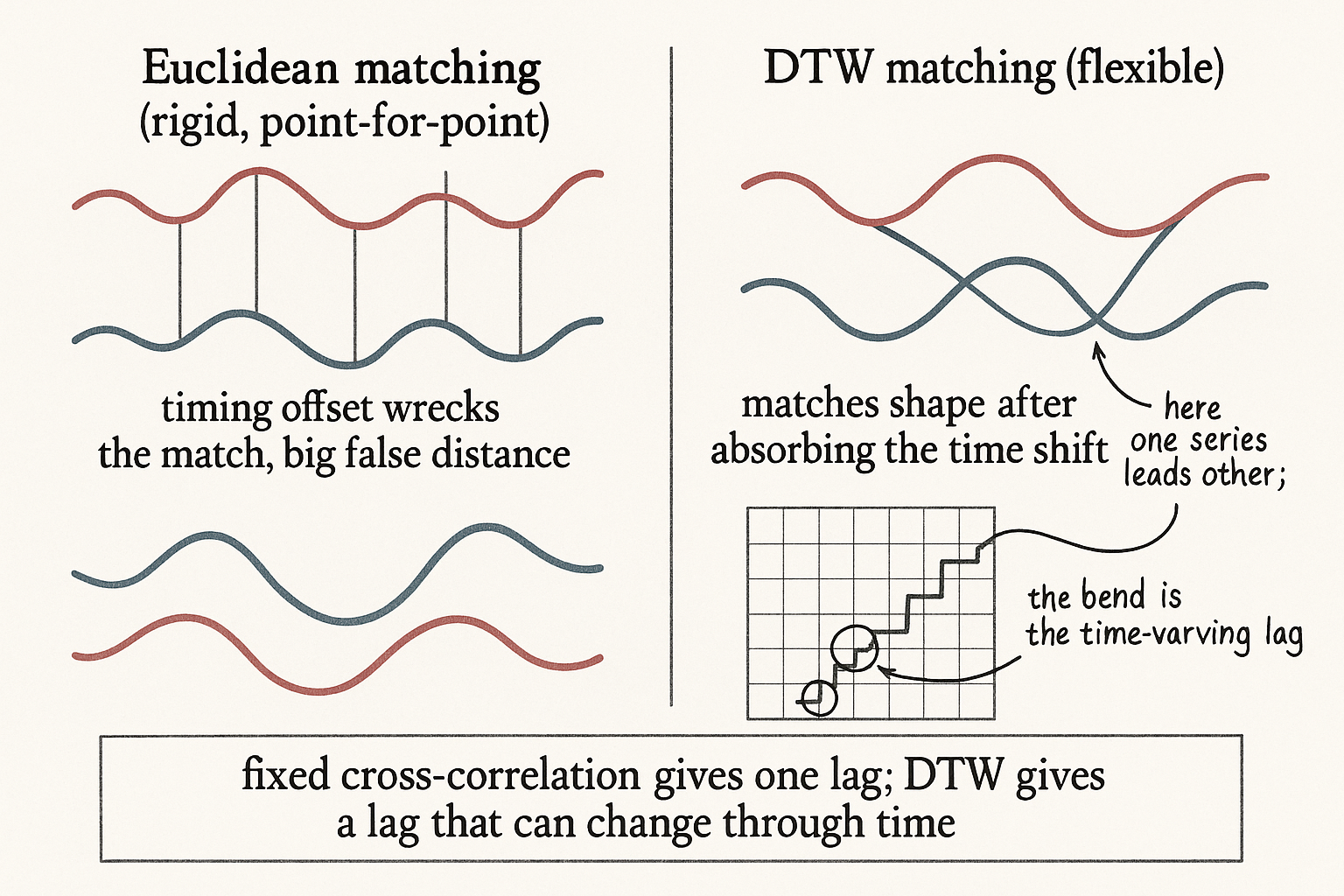
The default way to compare two series is to line them up index-by-index: A's first point against B's first point, second against second, and sum the gaps. That is Euclidean matching, and it assumes both series march on the same clock. If B is the same shape as A but shifted or stretched in time, Euclidean matching reports a huge distance even though the two are obviously the same pattern, because it is comparing A's peak against B's trough purely on account of a timing offset.
DTW throws out the one-to-one rule. It is allowed to match one point in A to several points in B, or skip ahead, whatever produces the cheapest total alignment. A point near A's peak gets matched to the point near B's peak even if they sit at different timestamps. The result is a distance that measures shape similarity after absorbing timing differences, which is exactly what you want when two markets trace the same move on a delay that wanders.
The recurrence
DTW is built from a cumulative cost matrix. Fill a grid where entry (i, j) is the cheapest total cost of aligning A up to point i with B up to point j, and build it with one short recurrence.
$$ D_{ij} = \left|A_i - B_j\right| \; + \; \min\!\left(D_{i-1,j-1},\; D_{i-1,j},\; D_{i,j-1}\right) $$
Read it left to right. The first term, the absolute difference between A's value at i and B's value at j, is the local cost of pairing those two points. The second term is the cheapest way to have arrived at cell (i, j) from its three predecessors: the diagonal step (advance both series one point), the vertical step (hold A, advance B), and the horizontal step (hold B, advance A). The diagonal is a normal one-to-one match; the vertical and horizontal steps are where the warping happens, one series waiting while the other catches up. Adding the local cost to the minimum of the three accumulates the best alignment so far. The number in the bottom-right corner, after filling the whole grid, is the DTW distance, and tracing the minimizing path back through the grid gives you the actual alignment, which point in A maps to which point in B.
That backtraced path is the lead-lag information you came for. When the path runs along the diagonal, the two series are moving in lockstep. When it veers horizontal or vertical, one is leading the other, and the size of the detour tells you by how much at that moment, a lag that varies through time instead of the single number the cross-correlation gives you.
The recipe in a few lines
The whole thing is a double loop over the cost grid. Code it once and you understand it better than any diagram.
import numpy as np

def dtw(A, B):
    n, m = len(A), len(B)
    D = np.full((n + 1, m + 1), np.inf)
    D[0, 0] = 0.0
    for i in range(1, n + 1):
        for j in range(1, m + 1):
            cost = abs(A[i - 1] - B[j - 1])          # local pairing cost
            D[i, j] = cost + min(D[i - 1, j - 1],      # diagonal: match
                                 D[i - 1, j],          # vertical: B waits
                                 D[i, j - 1])          # horizontal: A waits
    return D[n, m], D

def warping_path(D):
    i, j = D.shape[0] - 1, D.shape[1] - 1
    path = [(i, j)]
    while i > 1 or j > 1:
        step = np.argmin([D[i - 1, j - 1], D[i - 1, j], D[i, j - 1]])
        i, j = [(i - 1, j - 1), (i - 1, j), (i, j - 1)][step]
        path.append((i, j))
    return path[::-1]
The first function returns the DTW distance and the full cost matrix; the second walks the matrix backward from the corner, at each step taking whichever predecessor was cheapest, to recover the alignment. Run warping_path and plot the (i, j) pairs and you see the alignment bend wherever the lead-lag delay shifted.
Where it earns its keep, and where it costs you
The honest use cases are narrow and real. DTW gives you a similarity score between two assets that is robust to a wandering delay, which is a better input than raw correlation when you are clustering instruments by behavior or picking which pairs to even run a lead-lag study on, the graph-of-assets step the old lead-lag work used to choose what to trade. It also recovers a time-varying lag, telling you not just that A leads B but that the lead was short during calm and stretched during a fast move.
The costs are not small. The double loop is order n times m, quadratic in series length, so naive DTW on long high-frequency series is slow and you need a band constraint (forbid the path from straying too far off the diagonal) to make it tractable and to stop it from inventing absurd alignments. That band is also a guard against the deeper failure: unconstrained DTW will happily warp noise into a beautiful match, the same overfitting the old lead-lag article warned about when you scan too many pairs and lags, except now the model has even more freedom to find a pattern that is not there. And the warping path itself is not causal. It uses the whole series, future included, to decide the alignment, so it is a research and diagnostic tool for understanding a relationship, not something you drop straight into a live signal without a causal, online reformulation. Treat the distance as a similarity measure you trust and the path as a hypothesis about a varying lag you then verify out of sample, not as a tradable signal on its own.
Visualizing warping vs straight matching
KEY POINTS
- Lagged cross-correlation (the old article "Lead-Lag Relationships in Global Markets") assumes a constant delay between two series; real lead-lag delays wander, and a single fixed shift averages them into a blur.
- Euclidean matching compares two series index-by-index and reports a large distance for the same shape on a timing offset; DTW drops the one-to-one rule and matches each point to the corresponding point regardless of timestamp.
- DTW fills a cumulative cost matrix with D[i,j] = |A_i - B_j| + min of the three predecessors (diagonal = match, vertical/horizontal = one series waits); the corner value is the distance and the backtraced path is the alignment.
- The warping path is the payoff: diagonal stretches mean lockstep, horizontal or vertical detours mean one series leads, and the detour size is a lag that varies through time rather than one number.
- Good uses are a delay-robust similarity score for clustering assets and choosing pairs to study, plus recovering a time-varying lag, extending the lead-lag study from the old article "Crypto Cross-Exchange Lead-Lag Study."
- The costs are real: it is quadratic (needs a band constraint for long series), it overfits noise into pretty matches without that constraint, and the path is non-causal, so use it for research and diagnosis, not as a drop-in live signal.