9. Prediction Market Arbitrage July 1, 2026 6 min

9.14 Bayesian Edge in Log-Odds: Better, Earlier, Calibrated — or It's Noise

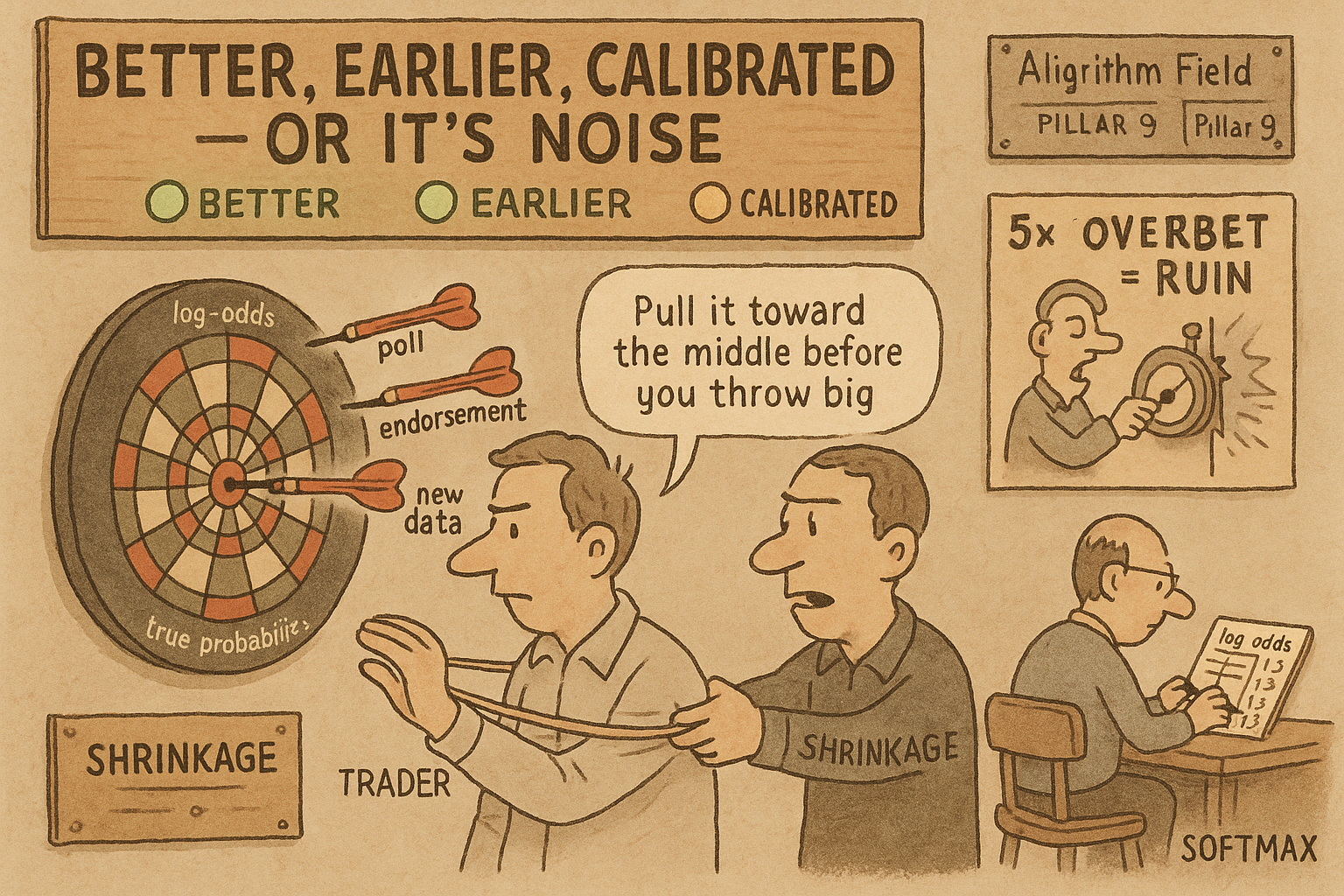
Bayes turns news into an edge, but the whole trade hangs on the likelihood ratio you estimate. Update in log-odds, tie it to the maker's softmax, and gate every belief on three tests: better, earlier, calibrated. Then shrink.

You passed the Brier Skill Score gate from the article on what a market price is. Your forecasts beat the market on historical resolutions. Now you want to turn a specific piece of news into a specific edge, and the tool is Bayes' rule. It is a clean update formula, and it is also where informational traders quietly destroy themselves, because the whole calculation hangs on a number you have to estimate and usually estimate too confidently. This article shows the update in the form that makes the danger visible, ties it to the market maker's own internals, and then spends most of its length on the three tests a belief must pass before it counts as edge.

The market price is your prior. Evidence moves it. The question is by how much, and the honest answer is smaller than you think.

Bayes as an update, worked

Start with the market price as your prior and let a poll arrive. Candidate A trades at $0.52, so the prior is 0.52. A poll shows A leading. You judge that poll is likely if A will win and less likely if A will lose.

$$ P(H \mid E) = \frac{P(E \mid H)\, P(H)}{P(E \mid H)\, P(H) + P(E \mid \neg H)\, P(\neg H)} = \frac{0.70 \times 0.52}{0.70 \times 0.52 + 0.25 \times 0.48} \approx 0.752 $$

Read that as: the posterior probability that A wins given the poll equals the likelihood of the poll under a win times the prior, divided by the total probability of seeing that poll either way, and plugging in a 0.70 likelihood under a win and 0.25 under a loss lifts the belief from 0.52 to about 0.752. That is a 23-point edge over the market, if the two likelihood numbers are right. They are the whole trade.

The odds form makes the danger visible

The fraction hides where the action is. Rewrite the update in odds and it becomes a single multiplication.

$$ \text{new odds} = \text{old odds} \times \text{likelihood ratio}, \qquad \frac{0.52}{0.48} \times \frac{0.70}{0.25} = 1.083 \times 2.8 = 3.033 \;\Rightarrow\; p = \frac{3.033}{1+3.033} \approx 0.752 $$

Read that as: convert the prior to odds, multiply by the likelihood ratio (how many times more likely the evidence is under the hypothesis than against it), and convert back, so the poll's entire effect is the factor 2.8. The edge lives in that ratio. Set the likelihood under a win to 0.70 when the truth is 0.55 and the ratio drops from 2.8 to 2.2, the posterior falls, and the edge you thought you had shrinks or vanishes. You did not misread the market. You misjudged one conditional probability, and the position sized on the inflated posterior is the belief-without-calibration failure from the article on the six ways to lose.

Sequential evidence adds in log-odds

Evidence rarely arrives once. In log-odds the update stops being a multiplication and becomes an addition, which is why this form scales.

$$ \operatorname{logit}\bigl(P(H \mid E_1,\ldots,E_n)\bigr) = \operatorname{logit}(P(H)) + \sum_{k=1}^{n} \ln\frac{P(E_k \mid H)}{P(E_k \mid \neg H)} $$

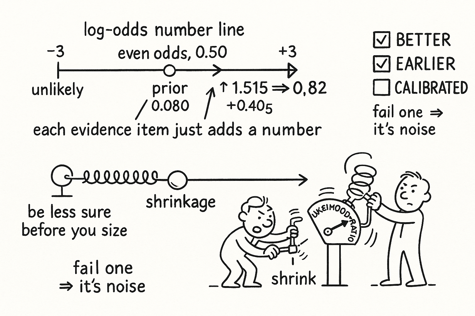
Read that as: take the log-odds of the prior and add, for each piece of independent evidence, the log of its likelihood ratio, so every new item just adds a number to a running total and you never reprocess old evidence. Work the example forward: the prior log-odds are the log of 0.52 over 0.48, about 0.080. The poll adds the log of 0.70 over 0.25, about 1.030. An endorsement with likelihood ratio 1.5 adds the log of 1.5, about 0.405. The total is 0.080 plus 1.030 plus 0.405, which is 1.515, and converting back gives about 0.820. Each item is one addition. This is not just convenient. The log-market-scoring-rule maker holds its state as exactly this log-odds vector and prices it with a softmax, the point the article on convex geometry makes about softmax being the price formula. Your Bayesian update and the market maker's pricing run on the same substrate. You are playing the maker's own game in the maker's own coordinates.

The true probability drifts: a filter on price

The event's real probability is not fixed. Campaigns, debates, and shocks move it, and the observed price is that moving target plus noise. A state-space model separates the two.

$$ x_t = f(x_{t-1}) + w_t \quad (\text{hidden true probability}), \qquad y_t = x_t + v_t \quad (\text{observed price}) $$

Read that as: the hidden true probability x evolves from its past value plus process noise w that represents genuine drift, and the price y you observe is that hidden value plus observation noise v from thin liquidity and noise trading. A Kalman filter estimates the hidden state and its residual, the filter's estimate minus the market price, is your trading signal: when the filter says the true probability has moved but the price has not caught up, that gap is temporal edge. For non-linear or non-Gaussian dynamics a particle filter does the same job with more flexibility. The old article "Volatility Regimes and Strategy Survival" frames the same idea of separating a slow-moving signal from fast noise; here the signal is a probability and the noise is microstructure.

When belief is not edge: three tests

A different posterior from the market is not automatically an edge. It counts only if it passes three tests at once.

Better: your likelihood model is more accurate than the market's implied one. If the crowd's conditional probabilities are sharper than yours, your update is worse than theirs and your "edge" is negative. Earlier: you process the evidence before the price moves. A correct update that arrives after the market already repriced is worth nothing, the exit-liquidity trap the article on execution covers. Calibrated: when you say 0.70 it happens about 70% of the time, the gate from the article on what a market price is.

Fail any one and the perceived edge is noise. The danger is asymmetric and it compounds through sizing.

$$ \text{true edge } 4\text{ pts, estimated } 20\text{ pts} \;\Rightarrow\; 5\times \text{ Kelly overbet} \;\Rightarrow\; \text{growth turns negative past a threshold} $$

Read that as: if the real edge is 4 percentage points but you estimate 20, Kelly sizes you five times too large, and because the growth penalty is quadratic in sizing error, overbetting past a threshold drives long-run growth below zero. This is why the article on the nine sources of edge ranks informational trading fifth and calls it the dangerous one: the edge estimate carries large uncertainty, and the penalty for overestimating is severe and one-sided. The old article "Ranking Beats Forecasting for Many Trading Problems" is worth holding in mind here, since a relative view is often more robust than an absolute probability estimate.

Shrinkage: the math of being less sure

When you suspect overconfidence, pull the forecast toward maximum uncertainty before sizing.

$$ p_{\text{shrunk}} = (1-\lambda)\, p_{\text{model}} + \lambda \cdot 0.5, \qquad \lambda = 0.3:\; 0.80 \to 0.7(0.80) + 0.3(0.5) = 0.71 $$

Read that as: blend your model's probability with a coin flip, weighting the coin flip by lambda, so a shrinkage of 0.3 turns an 80% forecast into 71%, a mechanical way to be less sure. The equivalent log-odds form divides your log-odds by one plus a regularization constant, collapsing toward 0.5 as the constant grows. Tune lambda to minimize your Brier score on a held-out set, and when in doubt shrink more, because underbetting is survivable and overbetting is not. Shrinkage is the direct antidote to the inflated-likelihood danger the odds form exposed: it caps how far a single overconfident conditional probability can push your size.

KEY POINTS

Bayes updates the market prior with evidence, but the whole edge lives in the likelihood ratio, a number you estimate. Overstate one conditional probability and the edge inflates or vanishes.
The odds form makes it plain: new odds equal old odds times the likelihood ratio. That single factor is the trade.
In log-odds the update is additive: each independent evidence item adds its log-likelihood ratio to a running total, no reprocessing needed. This is the exact substrate the log-market-scoring-rule maker uses, so your update and its pricing share coordinates.
The true probability drifts. A Kalman or particle filter on price separates signal from microstructure noise; the residual between filter estimate and price is temporal edge.
A different posterior is edge only if it is better, earlier, and calibrated at once. Fail any one and it is noise.
Overconfidence is lethal through sizing: a 4-point true edge estimated at 20 points is a 5x Kelly overbet, and the quadratic penalty turns growth negative. This is why informational edge ranks fifth and dangerous.
Shrink toward 0.50 before sizing, tune the shrinkage to minimize held-out Brier score, and when in doubt shrink more, because underbetting survives and overbetting does not.