A backtest is data, not a picture. The equity curve that comes out of a strategy run on historical prices is one observation drawn from a distribution of possible outcomes. The retail mindset stares at the curve, finds it beautiful, and ships the strategy. The experimental mindset treats the curve as a single sample and asks what would have happened under a thousand variations of the same world. The two approaches look identical up to the moment money is risked. After that they diverge violently.

The reason most live strategies disappoint is not that backtesting is broken. It is that most people do not run backtests as experiments. They run them as demonstrations.

What an experiment requires

A real experiment has six properties. Drop any of them and the result is decoration.

1. A pre-committed hypothesis. The rule, the parameter set, the universe of instruments, and the test window are written down before the test runs. No retrofitting after seeing the result.
2. A null hypothesis. What would the result look like if the rule had no predictive power? Without a null, "the rule made 14% per year" is a number with no reference frame.
3. Controlled inputs. No lookahead, no survivorship bias, no in-sample peeking, no parameters tuned on the same data used to evaluate. The test environment is as close to live conditions as the data allows.
4. A test statistic. One number that summarizes the outcome. Mean return per trade, Sharpe ratio, mean forward return after a signal. The same number is computed on the actual backtest and on every simulated null replication.
5. A sampling distribution. Some procedure that generates the distribution of the test statistic under the null. The procedure can be analytical (formulas) or computational (permutation, bootstrap, Monte Carlo). The sampling distribution is the reference frame that turns one number into evidence.
6. A decision rule. A p-value threshold or a confidence-interval criterion committed to before the test. Crossing the threshold is the rule for keeping the strategy. Failing to cross it is the rule for discarding it.

A backtest that fails any of these six checks is a screenshot. The equity curve might be true, but it is not evidence.

The two-component decomposition

Every backtest return decomposes into two parts.

Where R_backtest is the mean return per day observed in the test, R_predictive is the rule's true predictive contribution (positive, zero, or negative), β_bias is the rule's long/short bias (+1 = always long, −1 = always short, 0 = perfectly balanced), and μ_trend is the average daily return of the market during the test window.

The second term is free return from drift. It has nothing to do with the rule. A strategy that holds long 90 percent of the time during a period when the market drifted up at 0.05 percent per day collects 0.8 × 0.05% = 0.04% per day from drift alone. Over 252 trading days that compounds to roughly 10 percent per year of completely unearned return.

Worked example. Take a rule with zero predictive power applied to SPX from 2009 to 2021.

• The SPX had a positive net trend over the period. Average daily return ≈ 0.05%.
• The rule, by construction, is long 90% of the time and short 10%. β_bias = 0.8.
• Unwanted contribution = 0.8 × 0.05% = 0.04% per day.
• Annualized unwanted contribution ≈ 10%.
• The backtest equity curve looks great. Up 10% per year. Smooth.
• The rule has zero predictive power. Every cent of that 10% is drift × long bias.

In live trading this rule earns whatever the market drifts, minus slippage and costs. In a flat or down regime it loses money. The backtest never told the trader anything about the rule. It told the trader about the market.

The screenshot view sees +10% per year and ships the strategy. The experimental view detrends the data, recomputes the result, finds 0%, and discards the rule.

Detrending: removing the unwanted component

The fix is mechanical. Subtract the market's mean return from each day's return before running the rule on the data. The detrended series has zero net trend. Any positive return the rule produces on the detrended series is predictive power, not drift exposure.

Where R_t is the day's return and the bar denotes the sample mean over the full backtest window. Run the rule on R_detrended instead of R. Whatever performance comes out is the part that depends on the rule's signal timing, not on the wind being at its back.

This single adjustment kills more rules than any other validation step. It also keeps the rules that survive, because surviving on detrended data is a much harder bar.

One backtest is one sample

Even after detrending, a single equity curve is one observation drawn from a distribution. The same rule applied to a slightly different sample of the same market (different start date, different end date, different universe, different time of day) produces a different curve. The variation across those possible curves is the sampling variability, and it is what hypothesis testing measures.

The question "did the rule work?" needs a precise form. The precise form is: how often would chance alone produce a backtest at least this good?

To answer that, generate many fake versions of the world in which the rule has no predictive power. Permute the returns. Bootstrap them. Simulate paths with the same volatility and autocorrelation but no exploitable structure. Apply the rule to each fake version. Count what fraction of the fakes produce a result as extreme as the real one.

Where R_observed is the rule's actual detrended mean return, R*_i is the detrended mean return under the i-th permuted dataset, and N is the number of permutations. If p is below the threshold (0.05 is the convention), the actual result is unlikely under the null and the rule earns the benefit of the doubt. If p is above the threshold, the result is consistent with luck.

A backtest without this number is incomplete. A backtest with this number is an experiment.

Visualizing the screenshot vs the experiment

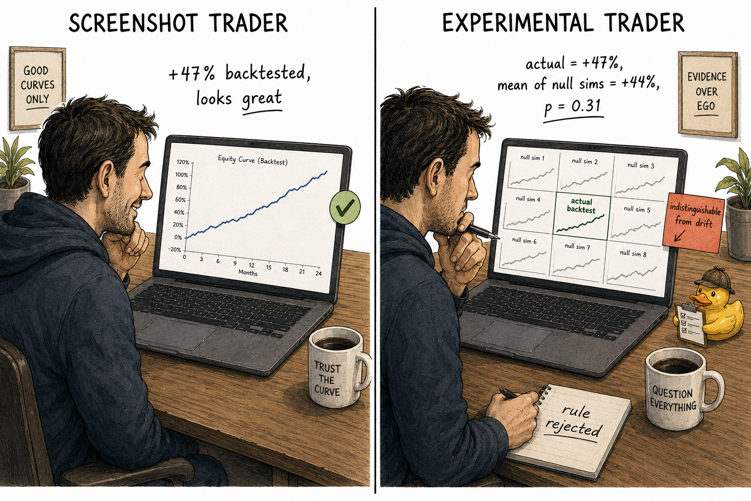
The screenshot view sees one curve and reads it as evidence. The experimental view sees one curve in the context of what chance alone would produce and reads the comparison as evidence.

The experimental backtest checklist

A backtest qualifies as an experiment when every item below is true.

1. The rule, parameters, universe, and test window are written down before the test runs.
2. The data is point-in-time accurate. No future information leaks into past decisions.
3. The market series is detrended, or returns are computed relative to a benchmark.
4. A test statistic is defined in advance (mean return, Sharpe, hit rate, profit factor).
5. A null model is defined in advance and is realistic (preserves volatility clustering, autocorrelation, and fat tails of the original series).
6. The null model is simulated enough times to estimate a p-value or confidence interval with low Monte Carlo noise. Five thousand replications is the floor.
7. The p-value or confidence interval is reported next to the headline performance metric.
8. The rejection threshold was committed to before the test ran.
9. If multiple rules or parameter combinations were tested, a multiple-testing correction is applied (Bonferroni, FDR, or a Reality Check style bootstrap).
10. The full pipeline is reproducible from raw data to final p-value given the code, the data, and the random seed.

A backtest that ticks all ten boxes can fail in live trading. A backtest that ticks fewer than ten almost certainly will.

What changes when this mindset is adopted

The number of rules that look good goes up. The number of rules that survive testing goes down. Most of the rules that get killed are the ones a trader would have most enjoyed running, because they were the ones with the highest screenshot equity curves and the lowest underlying predictive power.

The strategies that survive are unglamorous. Their backtested returns are smaller than the strategies that get discarded. Their confidence intervals are tight. Their p-values sit below the threshold. They make money in regimes where the rejected strategies would have collapsed.

The discipline is uncomfortable. The reward is that the strategies that ship behave in live trading the way they behaved in the backtest.

KEY POINTS

• A backtest is data, not a picture. The equity curve is one sample drawn from a distribution of possible outcomes under the rule.
• A real experiment requires six properties: pre-committed hypothesis, null hypothesis, controlled inputs, defined test statistic, sampling distribution, and decision rule.
• Every backtest return decomposes into a predictive component and an unwanted component (long/short bias × market net trend). The unwanted component can produce double-digit annual returns from drift alone with zero predictive power.
• Detrending the market series before running the rule removes the unwanted component. Performance on detrended data is the part attributable to the rule's signal timing.
• One equity curve cannot prove anything. Validity requires comparing the result to the distribution of outcomes under a realistic null model.
• The p-value is the fraction of null simulations that produce a result at least as good as the observed backtest. A backtest without a p-value or confidence interval is incomplete.
• The ten-item experimental backtest checklist (pre-committed parameters, PIT data, detrending, defined test statistic, realistic null, sufficient simulations, reported uncertainty, pre-committed threshold, multiple-testing correction, reproducibility) is the minimum viable protocol.
• Adopting the experimental mindset kills many strategies that look good. The ones that survive are the only ones worth running.