5.23 SAR: Seasonal Autoregressive Volatility Forecasting
SAR fixes vol seasonality by adding lags at 24 and 168 hours to an AR model, fit by OLS. The daily lag injects the midnight and 14:00 bumps a plain AR(1) misses, so you stop quoting tight into them.
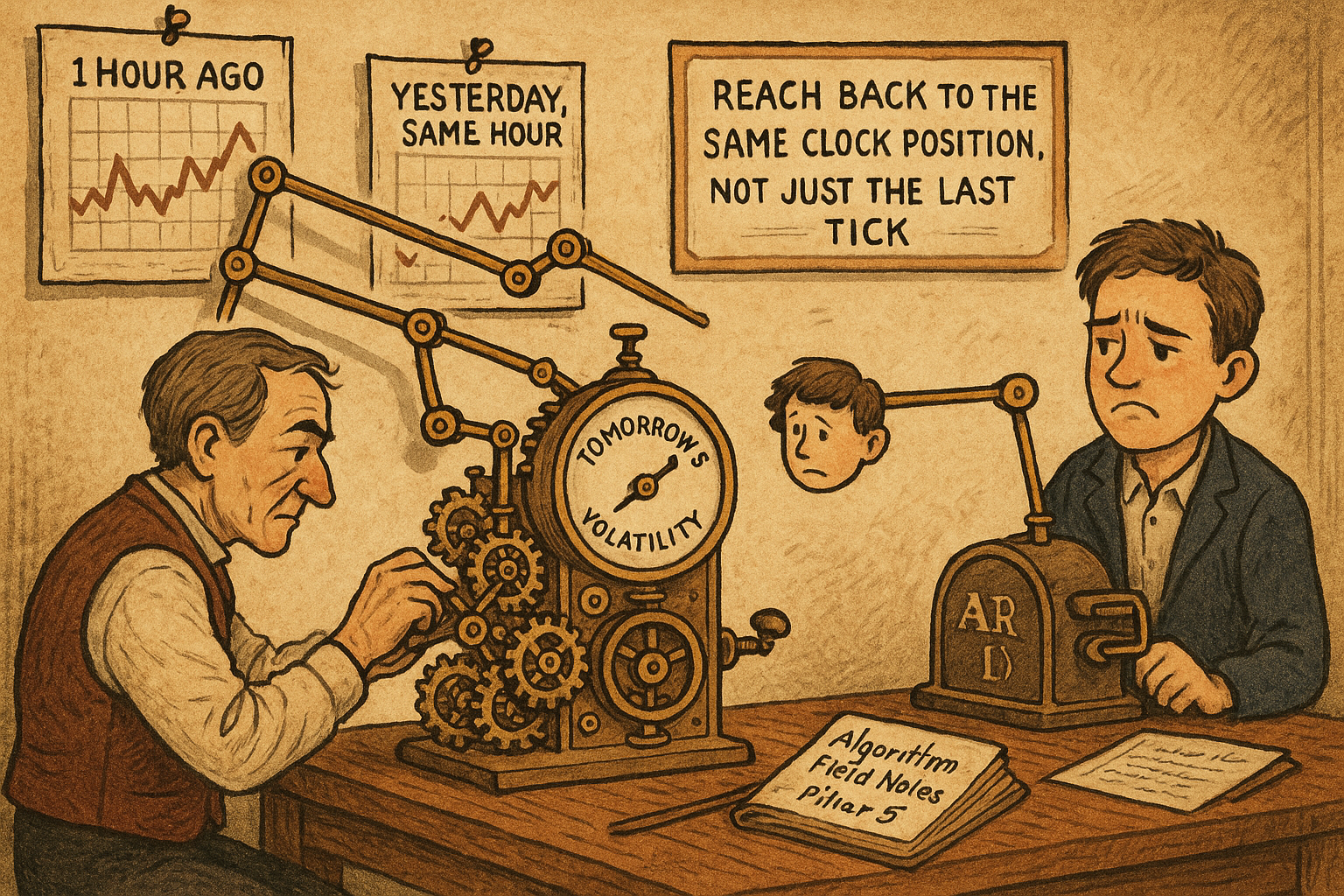
The old article "Crypto Volatility Seasonality" showed the bumps: vol clusters at 14:00 and 00:00 UTC, and the magnitude-only models walk right past them. This is the fix. Add lagged terms at the seasonal periods so the forecast can lean on "what did vol do at this same hour yesterday, and this same hour last week," not only "what did vol do an hour ago."
SAR stands for Seasonal Autoregressive. It is the plain AR model with extra lags placed at the periods where the series repeats. For hourly crypto vol the repeats are daily (24 hours) and weekly (168 hours), so those are the lags you bolt on. The model is a linear regression you fit by ordinary least squares, which means no special library and no excuse.
The model
Use squared hourly returns as the volatility proxy, the same proxy from the seasonality article. The forecast for the next hour's squared return is a constant plus three lagged squared returns: one hour back, 24 hours back, and 168 hours back.
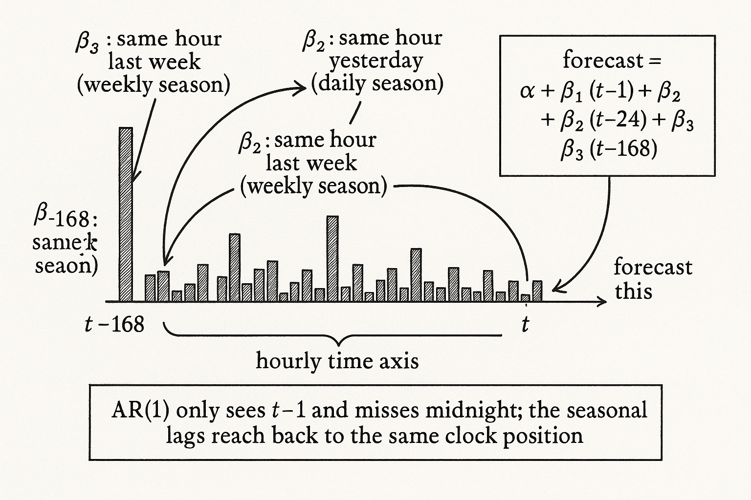
$$ \hat{y}^2_t = \alpha + \beta_1 \epsilon^2_{t-1} + \beta_2 \epsilon^2_{t-24} + \beta_3 \epsilon^2_{t-168} $$
Read each term in plain language. The epsilon-squared is the squared hourly return, the variance proxy. The alpha is the baseline variance the model falls back to when the lags carry no signal. Beta-1 on the one-hour lag captures the short-memory clustering that GARCH already gets: a violent last hour means a violent next hour. Beta-2 on the 24-hour lag is the daily seasonal term: it asks whether this same hour yesterday was loud, which is how the 00:00 and 14:00 bumps get into the forecast. Beta-3 on the 168-hour lag is the weekly term: weekends and specific weekdays trade differently, so the same hour one week ago carries its own information. The hat on the left is the predicted variance for hour t.
Fitting is multiple regression. Build a design matrix whose columns are the three lagged squared-return series, line up the target as the current squared return, and solve for alpha and the three betas by OLS. That is it. The seasonal lags are not a different estimator, they are extra columns in a linear regression.
A worked fit
Concrete numbers make the betas legible. Suppose OLS hands you alpha equal to a baseline variance matching a 30 bps hourly move, beta-1 of 0.25, beta-2 of 0.40, and beta-3 of 0.15. Now forecast the 00:00 UTC bar. The one-hour lag (23:00) was quiet, the 24-hour lag (last midnight) was a loud 70 bps move, and the 168-hour lag (midnight a week ago) was a 60 bps move. The forecast loads heavily on the 0.40 daily term hitting last midnight's large value, so the predicted vol for this midnight comes out well above the all-day baseline even though the immediately preceding hour was calm. A plain AR(1) sees only the calm 23:00 hour and forecasts low, then gets run over. The seasonal lags are what let SAR see midnight coming.
Note the betas usually rank the way intuition says: the one-hour term is strong (clustering is real), the daily term is the one that earns its keep on this series, and the weekly term is smaller and noisier. If beta-2 comes out near zero on your data, you do not have exploitable daily seasonality, and you should not force the term in because the seasonality article's plot looked suggestive. Let the regression tell you.
The other way to do it
There are two routes to the same place. One is this single regression with seasonal lags baked in. The other is a two-stage build: fit a plain AR(1) forecast on recent vol, then adjust that forecast up or down by a fixed seasonal factor for the current hour of day or day of week, the 24-point profile from the seasonality article. The two-stage version is easier to read and debug, because the seasonal adjustment is a separate multiplier you can inspect and the AR(1) part stays familiar. The single regression is cleaner statistically, because OLS sets all the weights jointly instead of you hand-tuning the split between "recent vol" and "seasonal factor." Pick the two-stage version when you want transparency, the joint regression when you want the fit to allocate the weight for you.
Either way this is the toy version. In production you would reach for S-GARCH, periodic GARCH, or a model that lets the conditional variance dynamics themselves change by season rather than just adding linear lags of squared returns. SAR is the honest minimum: it captures the seasonality the old article "Volatility Regimes and Strategy Survival" said you must respect, with a regression simple enough to fit in a few lines and audit by eye, and the old article "Why Volatility Is More Non-Stationary Than Trend" is the reason this is worth doing at all, since vol's long memory and structure are what the seasonal lags are pulling on.
Visualizing the lag structure
KEY POINTS
- SAR is plain AR with extra lags placed at the seasonal periods. For hourly crypto vol those are 24 hours (daily) and 168 hours (weekly).
- Forecast next hour's squared return as a constant plus three lagged squared returns: t-1, t-24, t-168. Fit alpha and the three betas by ordinary least squares; the seasonal lags are just extra columns.
- The 24-hour lag is the term that injects the 00:00 and 14:00 bumps into the forecast. A plain AR(1) sees only the immediately prior hour, forecasts low into a calm 23:00, and gets run over at midnight.
- Read the betas: clustering (t-1) strong, daily (t-24) the earner on this series, weekly (t-168) smaller and noisier. If the daily beta fits near zero, you have no exploitable daily seasonality, so do not force it in.
- Alternative two-stage build: AR(1) forecast times a per-hour seasonal factor. Easier to debug; the joint regression is cleaner because OLS sets the weights together.
- This is the toy version. Production uses S-GARCH or periodic GARCH that let the variance dynamics change by season, not just linear lags of squared returns.
References
- Seasonal Autoregressive (SARIMA) Models
- Periodic GARCH and Seasonal Volatility Modeling
- Forecasting Realized Volatility with the HAR Model
- Intraday and Weekly Seasonality in Cryptocurrency Volatility
- The Art of Currency Trading - Brent Donnelly (Amazon)
- A Comparison of Seasonal Adjustment Methods When Forecasting Intraday Stock Market Volatility
- A comparison of seasonal volatility models
- Modeling and Forecasting Realized Volatility
- Forecasting Realized Volatility: ARCH-Type Models vs. the HAR-RV Model
- Forecasting daily variability of the S&P 100 stock index using historical, realised and implied volatility measurements
- Forecasting Financial Market Volatility: A Review
- Understanding cryptocurrency volatility: The role of oil market shocks
- Correlations among cryptocurrencies: Evidence from multivariate factor stochastic volatility model