1.29 LLM Sentiment Trading: A Sharpe of Three That Needs an Autopsy
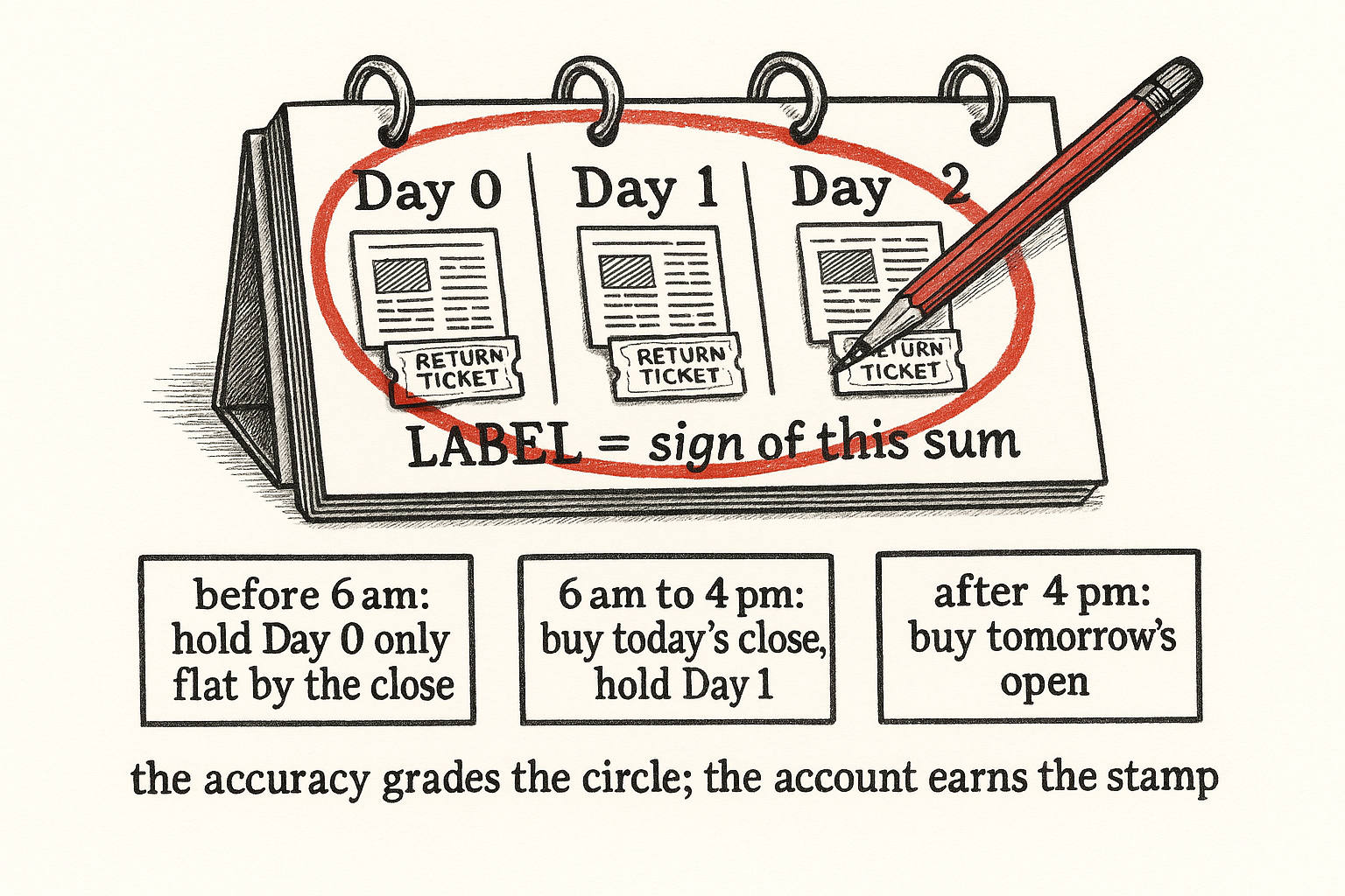
US stock LLM sentiment labels each article with the sign of the stock's three-day excess return. Date-split that label with a three-day embargo, or the accuracy grades the return it trained on.

Kemal Kirtac and Guido Germano take each US news article, label it with the sign of that stock's excess return on the publication day and the two days after, and fine-tune OPT, Meta's Open Pre-trained Transformer, which they treat as a public GPT-3-style model, to recover the label. The book is long the value-weighted top quintile of the score and short the bottom quintile, rebalanced every day, with a cost of 10 basis points (one tenth of one percent). The abstract's Sharpe ratio on that book is 3.05. The label is a sum of returns, and on part of the sample the fill sits inside the sum. A random split then lets the same three-day window train the score and grade it.
The label is the stock's own three-day excess return
They describe the label in prose and do not print the sum. Excess return on a day is the stock's return minus the market's return that day. The label sums the publication day and the two days after it, and the sign of that sum is the class. A positive sum is class 1. A zero or negative sum is class 0.
$$ e_{i,0:2} = \sum_{k=0}^{2} \left( r_{i,t+k} - r_{m,t+k} \right), \qquad y_i = \begin{cases} 1 & \text{if } e_{i,0:2} > 0 \\ 0 & \text{if } e_{i,0:2} \le 0 \end{cases} $$
The sum runs over the publication day and the next two trading days. The class is the sign, with a tie going to the negative bucket. Worked example. The stock returns 1.4%, then -0.2%, then 0.6%. The market returns 0.3%, 0.1%, and 0.4%. Excess returns are 1.1%, -0.3%, and 0.2%. The sum is 1.0%, which is positive, so the article is class 1. Flip the last stock return to -0.6% and the last excess is -1.0%, the sum is -0.2%, and the class is 0. The model is trained to recover that class from the text. The grade is the sign of the return path.
193,070 is the test slice, and they call it the training set
The sample after filters is 965,375 articles, from 2,732,845 Refinitiv items down to 1,865,372 that name one stock, then down again after a similarity screen, covering 6,214 firms from January 2010 through June 2023. They say they hold out 20% at random for testing, then 20% of what remains for validation, which leaves a training share of 64%.
$$ n_{\text{test}} = 0.20 \times 965{,}375 = 193{,}075, \qquad n_{\text{train}} = 0.64 \times 965{,}375 = 617{,}840 $$
The 20% slice is 193,075 articles. The training remainder their sentence describes is 617,840. The number they print as the training set is 193,070, five articles under the test slice and nowhere near 617,840. Keep both. The sentence names a training set and prints the test-set count. You cannot tell, from the paper, how many articles the model fit.
The cut is random. There is no date cut and no embargo. Monday's article and Tuesday's article on the same firm share two days of the three-day sum. A random draw puts Monday in the fit and Tuesday in the test, and the test article is scored on a return path the fit has already seen. The old article "How to Spot a Fake ML Trading Paper" is the checklist for this shape: an accuracy whose label is built from the series you then claim to forecast.
On the printed test metrics the confusion matrix is internally consistent, so the 74.4% agrees with the other three rates. They define accuracy as the share of articles whose class matches, precision as the share of predicted positives that are positive, recall as the share of positives that are caught, and specificity as the share of negatives that are caught. OPT prints accuracy 0.744, precision 0.732, recall 0.781, specificity 0.711.
$$ p = \frac{1 - \mathrm{specificity}}{\mathrm{recall}\,(1/\mathrm{precision} - 1) + (1 - \mathrm{specificity})} $$
That expression is the positive rate implied by the three rates, the fraction of articles whose three-day excess sum was positive. Plug in 0.711, 0.781, and 0.732. The numerator is 0.289. The first term in the denominator is 0.781 times (1/0.732 - 1), which is 0.286. Then p = 0.289 / (0.286 + 0.289) = 0.503. Rebuild accuracy as recall times p plus specificity times (1 - p): 0.781 times 0.503 plus 0.711 times 0.497 equals 0.746, against a printed 0.744. The F1 they define as the harmonic mean of precision and recall is 2 times 0.732 times 0.781, divided by 0.732 + 0.781, which is 0.756, against a printed 0.754. The cells agree with each other. The design is the problem.
OPT and BERT were fine-tuned on the label. FinBERT and the dictionary were not, on their account, and the four accuracies still sit in one table. OPT accuracy 0.744, BERT (Bidirectional Encoder Representations from Transformers) 0.725, FinBERT (a BERT already fit to financial text) 0.722, and the Loughran-McDonald dictionary (a finance word list scored by word counts) 0.501. The fine-tune lifts OPT by 0.022 over a model that, on their account, never saw the return label. A dictionary that never saw it sits on a coin flip. If the 0.722 is real, the wording of the article already lines up with the three-day sign before any return label is applied, which is what you get when the article describes a move that sits inside the sum. The extra 0.022 is the part that required the returns. The random split cannot tell those two stories apart.
The slope is 0.274, and most of the R-squared is dummies
After the classifier they regress the next day's stock return on the scores, with a firm intercept and a date intercept. They print the equation. Standard errors are clustered by firm and by date, so the t-statistic does not pretend that 965,375 articles are independent draws.
$$ r_{i,n+1} = a_i + b_n + \gamma \cdot x_{i,n} + \epsilon_{i,n} $$
The left side is the stock's return on the next trading day. a-sub-i is a firm intercept, b-sub-n is a date intercept, x is the score (a vector when more than one model is in the regression), gamma is the slope on that score, and epsilon is the residual. In the first specification, the one their caption and the grid agree contains two scores, the OPT slope is 0.274 with a t-statistic of 5.367 and the BERT slope is 0.142 with a t-statistic of 2.632. The regression is run on all 965,375 articles, including the rows the classifier was fit on. The score was fit to a three-day sum that includes this next-day return, and the regression then puts that same next-day return on the left side.
Worked plug-in, holding the intercepts fixed. Move the OPT score from 0.20 to 0.80 and the BERT score from 0.40 to 0.60. The change in the fitted return is 0.274 times 0.60 plus 0.142 times 0.20, which is 0.1644 plus 0.0284, so 0.1928 percentage points if the left side is in percent. That is 19 basis points for a large swing in both scores. One standard deviation of the OPT score, the 0.24 they print in the summary table, times 0.274 is 0.066 percentage points, about 7 basis points, with BERT held fixed.
The R-squared in that column is 0.221. The within R-squared, the fit after the firm and date intercepts have taken their cut, is 0.021.
$$ 1 - \frac{0.021}{0.221} = 0.905 $$
The score's piece is 0.021 out of 0.221, so 0.905 of the reported R-squared is the dummies. The adjusted R-squared in this column is 0.183, a real penalty. Firm and date dummies widen that gap. In four later columns the adjusted figure equals the raw figure. The caption says specifications 3 through 6 contain one score. In the paper text the grid puts OPT and FinBERT in the same column, puts FinBERT and the dictionary in another, and leaves the last column with no coefficient. Read the first column, where the caption and the cells agree. The other columns look misaligned, so leave them out of the trade.
The units of 0.274 have to be settled before the 19 basis points mean anything, because the summary table and the regression cannot be describing one return series.
$$ \left| \overline{r} - m \right| \le s $$
The left side is the gap between the mean daily return and the median, and s is the standard deviation. The gap cannot exceed the average distance from the observations to the median, because an average cannot sit farther from a point than the average distance to that point. The median minimizes that average distance, so the average distance to the median is no larger than the average distance to the mean. The average absolute distance to the mean cannot exceed the root-mean-square distance, which is the standard deviation. The standard deviation is therefore at least the gap between the mean and the median. Their summary table prints a mean daily return of 0.37%, a median of -0.02%, and a standard deviation of 0.18%, on the same 965,375 articles. The gap is 0.37 - (-0.02) = 0.39, and 0.39 is already larger than 0.18. The column fails a check every distribution satisfies. The minimum of -64.97% and the maximum of 237.11% only make a wide dispersion more plausible. They also call the scores normal around a median of 0.5 while printing an OPT mean of 0.53. Leave the cells as printed. The source may have the standard-deviation column wrong.
The regression's own RMSE in the first column is 5.32. A residual dispersion of 5.32 against a raw standard deviation of 0.18 would mean the fitted residuals are about 30 times wider than the series they came from. The summary table and the regression disagree on the scale of the return, and one of them has a bad cell. A Gaussian AIC on 965,375 observations with an RMSE of 5.32 is on the order of n times the log of the mean squared error, about 3.2 million. The table prints an AIC of 64,378. That cell disagrees with the sample size and the RMSE as well. The printed 0.18 stays, with the flag that it fails the mean-median check. Read the slope in the regression's units. An RMSE of 5.32 is a plausible daily stock residual in percent, and on that reading a slope of 0.274 is 27.4 basis points for a score that goes from 0 to 1.
A quintile book earns the slope times the gap between the top and bottom quintiles, a smaller move than a full swing from 0 to 1. They say the scores look normal. The mean of a standard normal above its 80th percentile equals the density at that percentile divided by 0.20.
$$ z_{0.80} = 0.842, \qquad \mathrm{E}[Z \mid Z > z_{0.80}] = \frac{\phi(z_{0.80})}{0.20} = 1.40 $$
The 80th percentile of a standard normal is 0.842, and the density there is 0.280. Divide by 0.20 and the top quintile sits 1.40 standard deviations above the center. The bottom quintile sits 1.40 below it. The gap in an OPT score with standard deviation 0.24 is 2 times 1.40 times 0.24 = 0.672. Times the slope 0.274, the fitted next-day gap is 0.184 percentage points, about 18 basis points a day. That calculation uses the normal they invoked. Their mean of 0.53 and median of 0.5 say the scores are not exactly normal, so treat 18 basis points as the slope's scale, not as a second backtest.
It also does not have to match the portfolio, and the reason is the intercepts. Firm intercepts remove a name that scores high every day and earns a high return every day. A value-weighted quintile still holds that name on the days it qualifies, and earns the name's return. Date intercepts remove the day. The sort can show a larger spread than 0.18 percent without anyone having misread the slope. A mean, a volatility, and a Sharpe still have to describe one strategy, and the equity curve still has to compound the mean.
The fill depends on which side of 6 am and 4 pm the article landed
The portfolio is value-weighted inside each leg. They describe the weights and do not print them. Top 20% of scores go in the long leg, bottom 20% in the short leg, weights proportional to market value inside the leg, reformed every day.
$$ w_i = \frac{v_i}{\sum_{k \in \mathrm{leg}} v_k}, \qquad R_{\mathrm{LS}} = \sum_{i \in L} w_i r_i - \sum_{j \in S} w_j r_j $$
Each name's weight is its market value over the market value of its leg. The long-short return is the long leg's return minus the short leg's stock return. Worked example. The long leg holds a name with market value 900 that returns +1.0% and a name with market value 100 that returns +6.0%. Weights are 0.90 and 0.10. The leg returns 0.90 times 1.0 plus 0.10 times 6.0, which is 1.50%. An equal weight would have returned 3.5%. The 6% name is a tenth of the leg, which is the point of value weighting: they say they want the large names, and the weight does that. The short leg holds market values 300 and 100 with stock returns -1.0% and +2.0%. Weights 0.75 and 0.25. The short basket's stock return is 0.75 times -1.0 plus 0.25 times 2.0, which is -0.25%. The long-short earns 1.50 - (-0.25) = 1.75% that day.
The clock decides which return those weights multiply. News before 6 am is bought at that day's open and sold the same day's close. News from 6 am to 4 pm is bought at that day's close and sold the next trading day. News after 4 pm is bought at the next open. The label, on every clock, still contains the publication day and the two days after it. The pre-6 am trade holds the open-to-close piece of the publication day and is flat before the two days that finish the label. The regression's left side is the next day, and that trade does not hold it. The midday trade buys the close, after part of the publication day's return is already in the article and in the label. The after-4 pm trade starts the next session, with the publication day entirely behind the fill and entirely inside the label. They pool the three clocks. They do not report the mix.
The similarity screen that built the 965,375 is also told two ways. The text drops an article whose cosine similarity with another article in the past 20 days is 0.8 or higher. The table caption says the window is the prior five business days. Same threshold, two windows. Leave both.
They charge 10 basis points "for each trade" and do not report turnover. A full replacement of both legs is four orders: sell the old long, buy the new long, buy to cover the old short, sell the new short.
$$ c = 0.001 \times \frac{T}{V} $$
The cost in fraction of net asset value is 10 basis points times dollars traded, divided by net asset value. Worked example, full replacement, one dollar long and one dollar short. Dollars traded are 4, net asset value is 1, and the cost is 0.40%, which is 40 basis points. A single 10 basis point haircut on the spread, once a day, is 0.10%, and 252 such days cost 25% of net asset value a year. Both readings use their 10 basis points. The turnover is unreported, so neither bill can be checked against the portfolio mean.
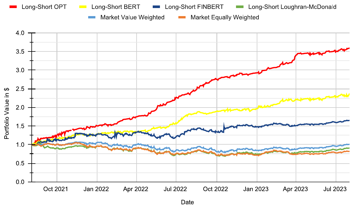
The red line ends near 3.6
Look at the red line. It is the OPT long-short. It starts at $1 and finishes near 3.6, under the 4.0 gridline.
Three Sharpes from the portfolio table, in the columns that put 3.05 on the OPT long-short the prose also names: OPT long-short 3.05, BERT long-short 2.11, FinBERT long-short 2.07. Those columns give OPT's long leg 1.81 and its short leg 1.42. The dictionary long-short is 1.23, which is the dictionary Sharpe the conclusion states.
The OPT long-short column also prints a mean daily return of 0.55% and a daily standard deviation of 2.49%. The long leg's mean is 0.32% and the short leg's is 0.25%. Those two add to 0.57, against the long-short's 0.55, so the three means belong in one column: the short leg's mean is a profit on the short, and the stocks in it fell. They print the Sharpe and the two inputs and do not print the annualization. The card is the usual scaling, mean over volatility, times the square root of the number of sessions in a year.
$$ SR = \frac{0.55}{2.49} \times \sqrt{252} $$
Mean daily return over daily standard deviation is the daily Sharpe, and multiplying by the square root of 252 is the annual figure on a stock-market calendar. 0.55 / 2.49 = 0.2209. The square root of 252 is 15.875. The product is 3.51. The table prints 3.05. The same 0.2209 times the square root of 365 is 4.22, against the printed 3.05. The day count that turns 0.2209 into 3.05 is (3.05 / 0.2209) squared, about 191 sessions. A year of sessions is 252 or 365, and 191 is neither. The long leg wants about 152 sessions to turn 0.32 / 2.18 into the printed 1.81. The short leg wants about 273 sessions to turn 0.25 / 2.91 into the printed 1.42. A single year-length would have produced one day count. The three columns produce three. The Sharpe column does not match the mean and volatility columns. The printed 3.05 stays, with the flag that the source's own cells disagree.
The equity curve is a second failure, and it does not depend on the annualization. Their prose window for the figure is August 2021 through July 2023. From 1 August 2021 through 31 July 2023 there are 521 weekdays, about 500 sessions once exchange holidays come out. The axis on the figure labels October, and the lines are already above 1 by then.
$$ W_{500} = (1.0055)^{500} = 15.53 $$
If every session earned the printed 0.55%, five hundred sessions turn $1 into $15.53, a gain of 1,453%. A log approximation that subtracts half the variance, using their 2.49% daily volatility, still finishes near 13.4. The red line finishes near 3.6.
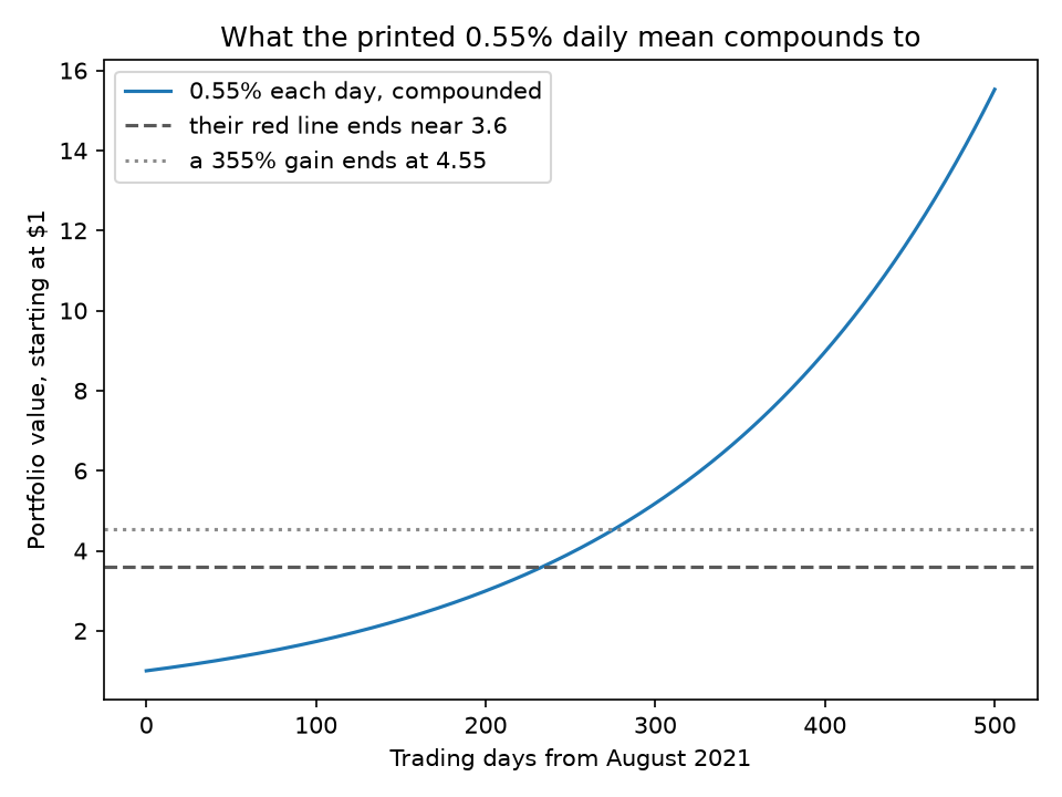
The abstract and the results section call the red line a 355% gain. A 355% gain finishes at 4.55, which is above the top of the chart the line never reaches. The conclusion calls the same strategy a 35% return, which finishes at 1.35, a level the red line leaves behind early. Reading the other lines off the same grid: BERT finishes near 2.3, a gain of about 130%, and the text says 235%. FinBERT finishes near 1.6, a gain of about 64%, and the text says 165%. The gaps are about 100 percentage points, which is what you get when the ending portfolio value is written down as a percent gain and the starting dollar is not subtracted. The dictionary line finishes near 0.90, a loss of about 10%, and the text calls that a 0.91% return. The value-weighted market finishes on the $1 line. The equal-weighted market finishes near 0.80. The text says the market portfolios barely exceed 1%.
The portfolio table does not name its window. Both ways of assigning one fail. If the 0.55% is the mean of the plotted window, the curve would have to end near 15, and it ends near 3.6. If the 0.55% is the mean of the sample they attach the Sharpe to, January 2010 through June 2023, that is 13.5 years, and 13.5 times 252 is 3,402 sessions. Raised to that power, 1.0055 becomes about 127 million. They do not plot that curve. They plot two years.
The dictionary's regression coefficient, 0.083 with a t-statistic of 1.871, carries no star under their rule that a star needs p below 0.05. The same paper gives the dictionary long-short a Sharpe of 1.23. The sort and the regression are not the same test, on the model they present as the weak one and on the model they present as the strong one.
Run the clock forward, or leave the book alone
Score the window you can hold, on articles whose entire three-day label ended before the test period starts. The embargo is three trading days, because that is the label. Train on earlier articles only. Report the three clocks separately: before 6 am, from 6 am to 4 pm, and after 4 pm, in exchange local time, using a timestamp you could have read before the fill. Charge 10 basis points on the dollars you traded, and print the turnover. Plot the book from January 2010 through June 2023. Put FinBERT and the dictionary through the same fine-tune as OPT, or through none. A slope you can recompute from the printed mean and volatility, as mean over volatility times the square root of 252, is the Sharpe you are allowed to quote.
The old article "Is Attention a Factor? WSB Herding, BERT Sentiment, and the Meme Confound" is this trap on a forum feed. A book of the loudest bullish names printed a factor-regression intercept of 0.433 percent a day, and the 20-day window after the shout, which is the window a holder earns, was an abnormal return of -0.045 percent. A fitted coefficient and a fill are different objects until you show they are the same days.
I am against funding the printed book. The condition under which the result would be a trade is the protocol above, on a later period, value-weighted, with the cost on the shares that turned over, and a Sharpe that matches its own mean and volatility. They did not run that test. What they ran is a classifier of a three-day return, scored on a random slice of the same years, and a two-year chart that does not compound the daily mean printed next to the Sharpe.
KEY POINTS
- Label the article with the sign of the three-day excess return. A positive sum is class 1, and that sum is the thing the accuracy grades.
- Split by date and check the count. The printed training set of 193,070 is five articles under 20% of 965,375. A 64% training share is 617,840.
- Read the within regression before the R-squared. The OPT slope is 0.274, about 7 basis points per standard deviation of the score, and the within R-squared is 0.021.
- Clock the fill. Before 6 am you are flat the same day, and the label still contains the next two days.
- Recompute the Sharpe from the printed mean and volatility. 0.55 divided by 2.49, times the square root of 252, is 3.51, and the table prints 3.05.
References
- How to Spot a Fake ML Trading Paper
- Is Attention a Factor? WSB Herding, BERT Sentiment, and the Meme Confound
- Sentiment trading with large language models (Kemal Kirtac and Guido Germano)
A note on AI. The ideas, research, analysis, and conclusions in this article are my own. I use AI tools to help with editing and wordsmithing, because English is not my first language, and I am not shy about that. AI-generated ideas and AI-assisted writing are not the same thing: the first is empty slop from a generic prompt, the second is a tool for communicating years of real research more clearly. Judge the work by its substance, not by whether software helped polish the prose.