3.46 Mean-Reverting Stat-Arb in Crude Oil: WTI vs Brent/Dubai
Crude-oil statistical arbitrage fades the WTI minus Brent/Dubai residual with a power of the gap. Re-fit the hedge ratios when a break test rejects stable weights.
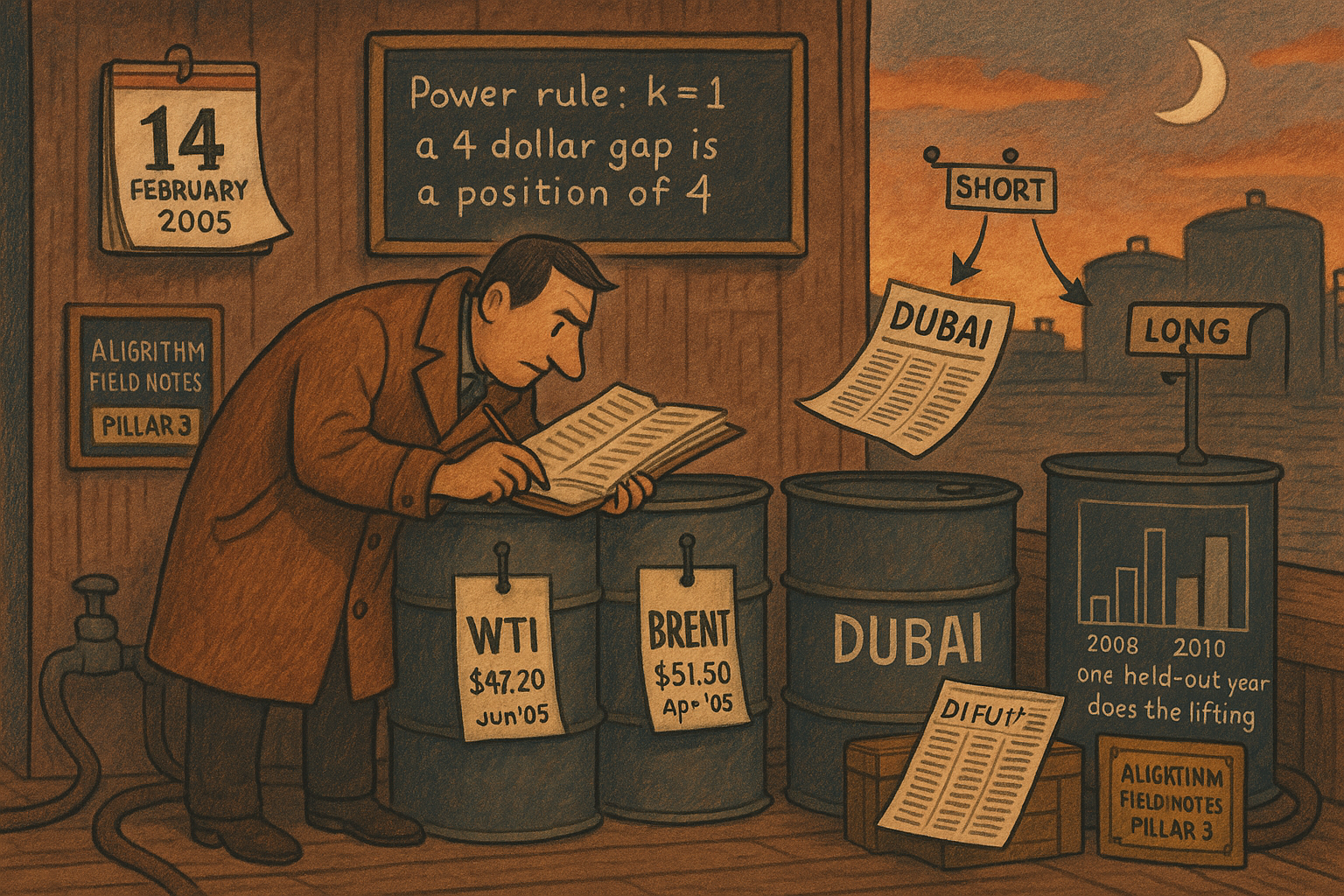
Fanelli defines a statistical arbitrage as a zero-cost book whose expected value at a fixed horizon is at least zero, and whose conditional variance of that terminal value falls as the clock runs. On crude she builds that book as West Texas Intermediate futures against Brent and Dubai. The Brent and Dubai weights come from a cointegration regression, and the regression prints an R-squared of 0.995. The residual from the fit is the mispricing. She fades it with a power rule: the position takes the opposite sign of last week's residual, and the size is a power of how far that residual sat from zero.
Terminal variance has to fall
Three conditions have to hold at a horizon T. The book starts at zero value. Its expected value at T, given what was known at the start, is at least zero. And the variance of that same terminal value, given the information at an intermediate date t, falls as t moves forward. A drift toward a positive level, with the error band on the terminal payout shrinking, is the whole definition. The remark she attaches describes pure arbitrage as the stronger demand that the terminal value be non-negative in every state.
She writes the mispricing M as an Ornstein-Uhlenbeck process. Alpha is the speed of mean reversion, in units of one over time. Theta is the level M is pulled toward. Sigma is the shock volatility. W is a Brownian motion. The process is started at zero.
$$ dM_t = \alpha(\Theta - M_t)\,dt + \sigma\,dW_t, \qquad M_0 = 0 $$
Alpha of 0.2 per week is a half-life of 3.47 weeks, because ln(2) divided by 0.2 is 3.47: that is how long a gap takes to close halfway to theta. Theta of 1 is a pull toward 1 dollar of mispricing. Sigma of 0.5 is half a dollar of shock per square-root week. She never estimates alpha, theta, or sigma on the oil residual. The arithmetic below is this chosen process, so the definition can be recomputed.
Given the value at an earlier time s, the mean and variance at a later time t are closed form.
$$ E[M_t \mid \mathcal{F}_s] = \Theta + (M_s - \Theta)e^{-\alpha(t-s)}, \qquad Var[M_t \mid \mathcal{F}_s] = \frac{\sigma^2}{2\alpha}\left(1 - e^{-2\alpha(t-s)}\right) $$
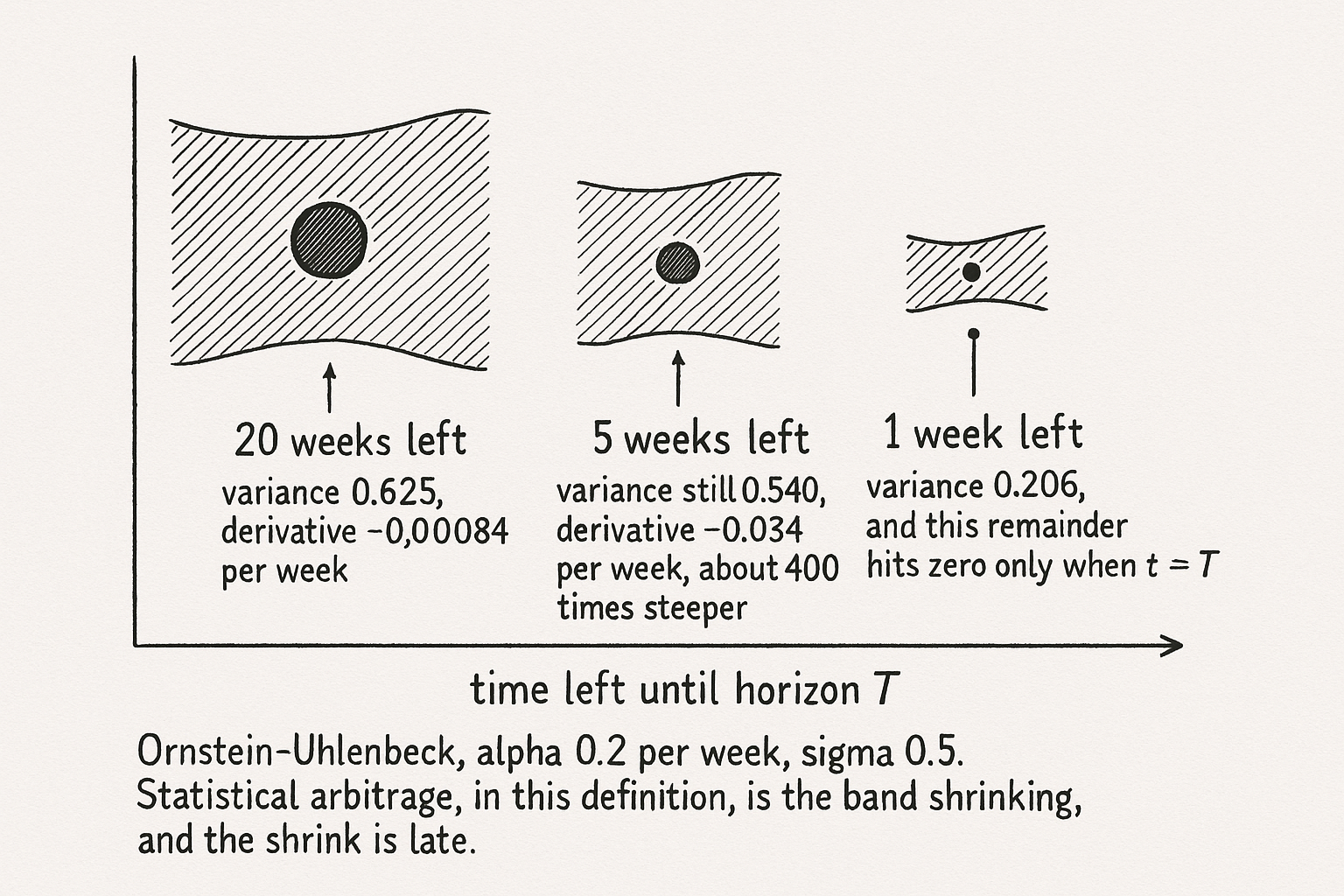
The mean is theta plus whatever gap is left, decayed by the exponential. The variance grows toward sigma-squared over 2 alpha as the gap between s and t gets long. It is a function of that time gap alone. Start at 0 and set T to 20 weeks. The expected terminal value is theta times (1 minus e to the minus alpha T), which is 1 minus e to the minus 4, which is 0.982. The variance of that terminal value, seen from week 0, is (0.25 / 0.4) times (1 minus e to the minus 8). Sigma-squared over 2 alpha equals 0.625, and e to the minus 8 is 0.0003, so the variance is 0.625.
The definition requires this variance to fall as t rises. Differentiate the terminal variance with respect to t.
$$ \frac{\partial}{\partial t} Var[M_T \mid \mathcal{F}_t] = -\sigma^2 e^{-2\alpha(T-t)} $$
The derivative equals minus sigma-squared times an exponential in the time still left. With sigma at 0.5 it is strictly negative at every t before T. At week 0, with 20 weeks left, it is minus 0.25 times e to the minus 8, which is minus 0.000084 per week. At week 15 the variance has only moved from 0.625 to 0.540, and the derivative is minus 0.034 per week, about 400 times steeper. With one week left the variance is still 0.206. That 0.206 has to reach zero in the last week, because once t equals T the terminal value is known. The decline she invokes is real, and almost all of it shows up at the end of the horizon.
The same formulas with a different start keep the variance condition and lose the positive-expectation condition. Start at M equal to -2 and look five weeks ahead. The expected value is 1 plus (-2 minus 1) times e to the minus 1, which is 1 minus 3/e, which is -0.104. The derivative of the variance has no M in it, so it is still negative. The proposition gets a positive expected terminal value by pinning the start at zero and theta above zero. Her plotted crude residual runs from about -4 to about +7. At those levels, whether the expected terminal value is positive depends on the horizon you pick, the way the -0.104 case does.
The basket is a regression of WTI on Brent and Dubai
The mispricing you can build from prices is WTI minus a constant minus a weighted Brent and a weighted Dubai. Z is the WTI future, v1 is Brent, v2 is Dubai. The constant c and the weights h1 and h2 are the cointegration regression.
$$ M_t = Z_t - \left(c + h^{1} v^{1}_t + h^{2} v^{2}_t\right) $$
You are long one WTI, short h1 Brent, and short h2 Dubai. A negative h2 is a long Dubai leg. On the full weekly sample, 461 observations from 25 October 2000 to 19 October 2009, she prints c = 1.61763, h1 = 1.19378, and h2 = -0.21702. Put all three crudes at 50 dollars. The fitted WTI is 1.61763 plus 1.19378 times 50 plus (-0.21702) times 50, which is 1.61763 plus 59.689 minus 10.851, which is 50.46. The note under that table writes a minus in front of each weight. Those same coefficients with the minus fit WTI at 1.61763 minus 59.689 minus (-10.851), which is -47.22. A fitted price of -47 dollars in a 50 dollar market is the regression running the wrong way. The daily section of the same paper writes the plus form, and the portfolio prose is long WTI against the weighted basket, which is the plus form again. Use the plus form. The minus in the weekly note is a candidate for a source error.
The fit is tight in the way a common trend is tight. R-squared is 0.99515. The standard error of the regression is 1.83 dollars a barrel. The Durbin-Watson statistic, a measure of residual autocorrelation, is 0.256805. The usual AR(1) reading is one minus half of that statistic: 1 minus 0.12840 equals 0.872. A weekly autocorrelation of 0.872 has a half-life near five weeks, ln(0.5) divided by ln(0.872). An R-squared of 0.995 sitting on a Durbin-Watson of 0.26 is a shared trend plus a slow residual. The augmented Dickey-Fuller statistic on the residual, the unit-root test, is -3.75, with a p-value of 0.049. She treats that p-value as a weak stationarity result and moves on to a variance ratio.
Two other cells in the same table disagree with the numbers printed beside them. The Brent coefficient 1.19378 divided by its standard error 0.04061 is 29.40. The table prints a t-statistic of 9.40. The intercept ratio is 1.61763 over 0.19417, which is 8.33, and it matches the printed t-statistic. Dubai's ratio, -0.21702 over 0.04222, is -5.14, and it matches too. The F-statistic is printed as 47.012. From an R-squared of 0.99515, 461 rows, and two regressors,
$$ F = \frac{R^{2}/2}{(1-R^{2})/(461-3)} = \frac{0.99515/2}{0.00485/458} = 46987 $$
The printed F and the printed R-squared cannot both be right. A root-mean-square error of 0.0306 is printed under a regression standard error of 1.83 dollars. Divide 1.832739 by 0.030600 and you get 59.9. In the same units the root-mean-square error and the standard error differ by the degrees-of-freedom factor sqrt(461/458), which is 1.003, so they would both be about 1.83. Keep the coefficients. Skip the printed F and the printed Brent t-statistic.
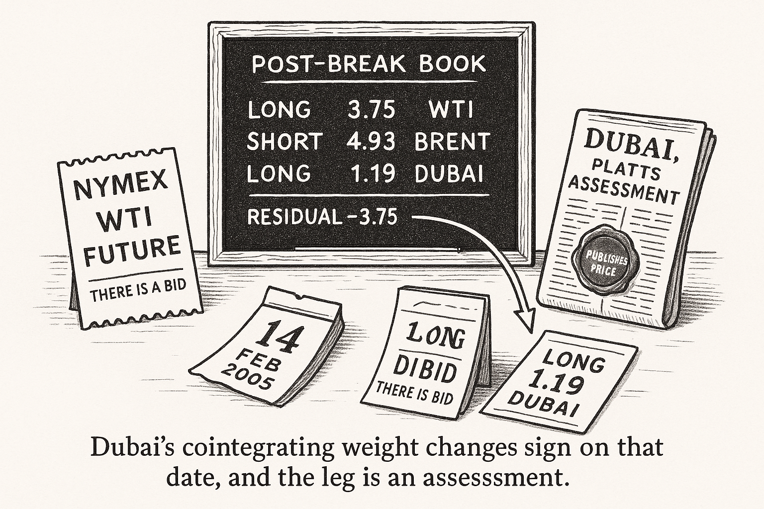
She then runs a Quandt likelihood ratio test: the maximum, over the central 70 percent of the sample, of the Chow statistics for a break in the intercept and both slopes. The statistic is 61.27. She rejects stable coefficients at the 1 percent level and dates the break at 14 February 2005. The old article "Why Systems Work Until They Don't" is the frame for what you do next. A hedge ratio that changes sign is a different book after the date, and the backtest has to be told the date. Before the break the constant is -2.229, the Brent weight is 0.976, and the Dubai weight is 0.185, so both Brent and Dubai are shorts. After the break, on the window through 31 December 2007, the constant is -1.078, the Brent weight is 1.316, and the Dubai weight is -0.317. The Dubai leg has moved to the long side.
Work those post-break weights at WTI 70, Brent 74, and Dubai 71. Fitted WTI is -1.07760 plus 1.31559 times 74 plus (-0.317238) times 71. That is -1.07760 plus 97.354 minus 22.524, which is 73.75. The residual is 70 minus 73.75, which is -3.75 dollars. WTI is cheap to the basket by 3.75. At a power of 1 you buy 3.75 units of the mispricing. The legs are long 3.75 WTI, short 3.75 times 1.31559 which is 4.93 Brent, and long 3.75 times 0.31724 which is 1.19 Dubai.
The gap she describes in words and the break date the test returns land in different years. The residual, she writes, fluctuated inside a band of -2 to +2 dollars through the end of 2006. The visible Brent premium came after that, with an average gap of 4.23 dollars a barrel in February 2009. The coefficient break is February 2005. Johansen's trace test splits the same way. Before the break the p-value on the hypothesis of no cointegration is 0.077. After the break it is 0.004. The post-break adjusted R-squared is printed as 0.972 next to an R-squared of 0.982, and the Durbin-Watson statistic on that same table is also 0.972. On about 150 weeks, February 2005 through December 2007, an R-squared of 0.982 still adjusts to 0.982. The gap that was printed, (1 minus 0.972) divided by (1 minus 0.982), equals 1.56. For a three-parameter regression that ratio equals (n minus 1) over (n minus 3), which solves near n = 7.
The old article "Stocks and Bonds Predict FX — But Only in Emerging Markets" asks when prices in one market forecast another. Fanelli's regression is contemporaneous. Brent and Dubai hedge WTI on the same date, and the position is in the residual. A high R-squared across related markets still has to pass a break test, and this regression's break test rejects stable weights.
On the daily sample she writes the plus form from the start. Using 1 January 2010 through 25 April 2017, the constant is 23.88 dollars, the Brent weight is -0.040 with a t-statistic of -0.50, and the Dubai weight is 0.730 with a t-statistic of 8.18. The daily basket is the Dubai term plus that 23.88 dollar constant. The old article "Stat-Arb Is a Clustering Problem: Multi-View Spectral > Any Signal" puts the result on which names share the basket. Brent's daily t-statistic says Brent is out. A second Quandt test dates a break at 1 June 2011. She attributes that date to Cushing storage, the GSCI cutting WTI's weight and raising Brent's, Libya, and Fukushima, and she says the coefficients change there. She does not print the split daily weights.
The variance ratio drops below one
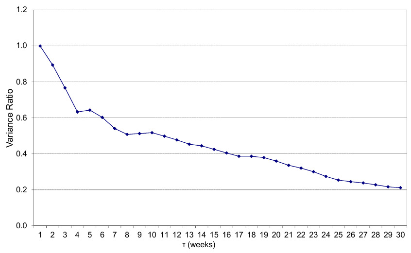
The Dickey-Fuller p-value of 0.049 is too close to the 5 percent line to carry a mean-reversion claim, and she says as much. The check she uses is the variance ratio at horizon tau. She describes it as the normalized ratio of the long-horizon variance of the mispricing to the single-period variance. She does not print the expression. The normalization whose random-walk benchmark is 1, which is the cutoff she uses (above 1 she calls trend, below 1 she calls reversion), is the usual divisor of tau.
$$ VR(\tau) = \frac{Var(M_t - M_{t-\tau})}{\tau \, Var(M_t - M_{t-1})} $$
The numerator is the variance of a tau-week change in the residual. The denominator is tau times the variance of a one-week change. A random walk sits at 1. Read off her figure: the ratio is 1 at one week, about 0.5 at eight weeks, and about 0.2 at thirty weeks, with a small uptick between week 4 and week 5. Take the one-week variance as v. An eight-week ratio of 0.5 means the eight-week variance is 0.5 times 8 times v, which is 4v, against 8v on a random walk. A thirty-week ratio of 0.2 means the thirty-week variance is 6v, against 30v. The long difference has about one fifth of the variance a random walk would have accumulated. That is mean reversion in the series plotted. The series is a residual whose hedge ratios the Quandt test has already rejected, so the ratio describes that constructed series. The weights under it change in February 2005.
The position is a power of last week's gap
The power rule sets today's position from last week's residual. The sensitivity k decides how hard the size grows with the gap. At k equal to 0 the position is a step of one unit, long or short. At k equal to 1 the position equals the residual with the sign flipped. She notes that k above 1 loads even harder on large gaps. The grid she searches runs only from 0 to 1.
$$ S_t^{k} = -\operatorname{sign}(M_{t-1})\,|M_{t-1}|^{k} $$
The sign function is the sign of last week's residual, and the absolute value is raised to k before the leading minus flips the side. A residual of +4 dollars, rich WTI. At k equal to 0 the position is -1. At k equal to 0.5 it is -2. At k equal to 1 it is -4. The signal is the same gap. k equal to 1 holds four times the unit position. A cumulative-profit ranking that puts k equal to 1 first, which is what her raw-rule plot does for k of 0, 0.5, and 1, is mostly ranking a larger bet on the same residual.
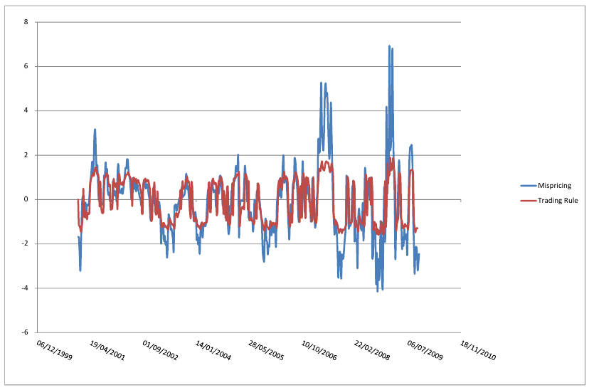
The figure she draws for the rule uses k equal to 0.33. A gap of 7 raised to 0.33 is 1.90. The red line peaks near 2 when the blue line peaks near 7, and the peak is on the same side of zero. The leading minus in the formula would put that peak near -1.90. The plotted series has the amplitude of the power and the sign of the mispricing. Either the figure drops the minus, or the red line is the negative of the formula. Her instruction is to sell the book when the signal is negative. On the series as plotted, a negative red line is a negative residual, so that sale shorts WTI on a week when WTI is already cheap.
Two dampers sit on top of the power. The moving average is the mean of the previous h power signals. The sum runs over j from 1 to h, so it is yesterday's signal back through h weeks, and today's power signal is outside it.
$$ S_t^{h} = \frac{1}{h}\sum_{j=1}^{h} S_{t-j}^{k} $$
Five previous signals, -1, -1.5, -2, -3, and -4, sum to -11.5 and average to -2.3. Today's raw signal can already be -4. The average you would trade is still -2.3.
The smoother then mixes today's power signal with yesterday's smoothed position. O is the weight on yesterday's position. Her grid runs O from 0 to 0.75.
$$ S_t^{O} = (1-O)\,S_t^{k} + O\,S_{t-1}^{O} $$
Start from a smoothed position of -1, with today's power signal at -4. At O equal to 0.5 the new position is 0.5 times -4 plus 0.5 times -1, which is -2.5. At O equal to 0.8, the setting in her three-strategy picture, it is 0.2 times -4 plus 0.8 times -1, which is -1.6. A larger O stays closer to the position already on, which is how she cuts the number of transactions. The weekly formula applies this mix to the power rule. The daily formula nests a 6-week moving average in place of the power signal, with k equal to 1, h equal to 6, and O equal to 0.5. The caption on the weekly comparison picture also feeds an h of 5 into the smoother. The weekly equation, the daily equation, and that caption are three recursions.
Weekly profit is the faded gap over the gross price
The week's mark is the position times the change in the residual, divided by the gross of the WTI price and the basket value, minus a charge on the change in position. Delta M is this week's residual minus last week's. Delta S is this week's position minus last week's. The cost rate c is 0.0025 in the backtest. V is the value of the Brent and Dubai basket.
$$ R_t = S_t^{k}\,\frac{\Delta M_t}{Z_t + V_t} - c\,|\Delta S_t^{k}| $$
In December 2024 she corrected this line. The price in the denominator is the WTI price Z. An earlier printing had put the position S in that slot, and in the sentence under the equation. She writes that the conclusions stand. The expression above is the corrected one.
Work a week with stated inputs, separate from her tape. The position is -2. The residual falls by 0.80 dollars. The gross Z plus V is 160. The first term is -2 times -0.80, divided by 160, which is 0.010. The position moved from -1 to -2, so the absolute change is 1, and the cost is 0.0025. The mark is 0.0075. If the residual widens by the same 0.80, the first term is -0.010 and the mark is -0.0125. The fade has to show up. The cost term multiplies the change in position. The barrel price is absent from that term. Apply the same 0.25 percent to a 70 dollar barrel and you get 17.5 cents, which is 17.5 WTI ticks at 1 cent a tick. Her formula's charge for a one-unit change in position is 0.25 percent of the mark, at any barrel price. The paper leaves the two readings unspecified.
The total return in the tables is the sum of these weekly marks. The Sharpe ratio she prints is the mean mark divided by the root-mean-square deviation of the marks. Both the mean and the variance divide by t, the number of weeks. The formula subtracts nothing for funding. The prose calls the numerator an annualized mean profitability and the denominator an annualized standard deviation.
$$ \Pi_t = \frac{\frac{1}{t}\sum_{s=1}^{t} R_s}{\sqrt{\frac{1}{t}\sum_{s=1}^{t}\left(R_s - \frac{1}{t}\sum_{s=1}^{t} R_s\right)^{2}}} $$
The square-root-of-weeks factor that would turn a weekly ratio into an annual one is absent. Three illustrative weeks, 0.010, -0.004, and 0.007, sum to 0.013. Divided by 3 the mean is 0.004333. The root-mean-square deviation, dividing by 3, is 0.006018. The ratio is 0.72. That is what the formula returns. Whether a table entry of 0.85 is this object or the annualized ratio the prose describes is a question about the results, taken up next.
2009 carries the out-of-sample result
The hatched bars are 2008, 2009, and 2010, the years she holds out. Look at 2009. The other tall bar is 2007, and 2007 is still inside the fit.
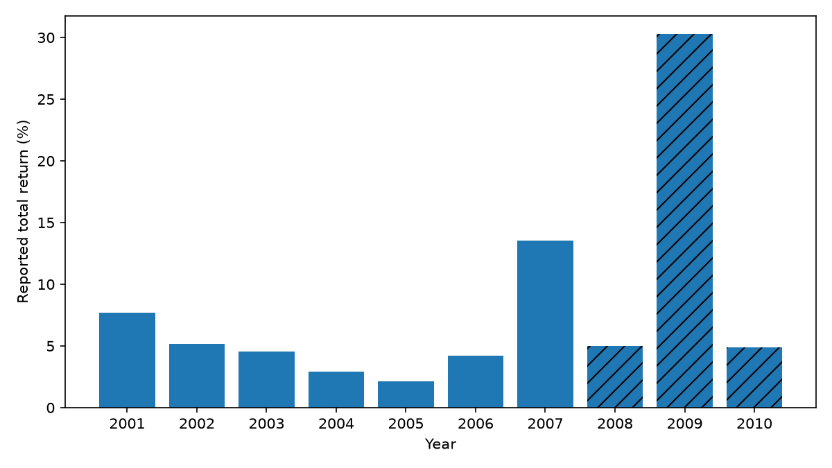
Out of sample, on the smoothed rule at k equal to 1 and a cost of 0.25 percent, the reported total returns are 4.97 percent in 2008, 30.26 percent in 2009, and 4.90 percent in 2010. The Sharpes on those years are 0.85, 0.69, and 0.80. Across the seven in-sample years the total return averages 5.75 percent, ranging from 2.14 percent to 13.53 percent, and the Sharpe falls from 1.70 in 2001 to 0.85 in 2007; the out-of-sample shares of profitable weeks are 42.31 percent, 57.14 percent, and 50.00 percent. The daily tables print 20.34 percent for 2014 and 13.84 percent for 2015, both beside a row labeled Shape ratio at 0.86, while the note treats 2014 as in-sample and the stated out-of-sample window runs from 2015 through 10 April 2017, years the table leaves out.
Put the weekly Sharpe next to both readings of her definition. If 0.85 is already the annualized ratio the prose describes, 2008's volatility is 4.97 divided by 0.85, which is 5.85 percent, and 2009's volatility is 30.26 divided by 0.69, which is 43.86 percent. If 0.85 is the raw weekly ratio the formula prints, and a year's total return is the sum of 52 weekly marks, then annualized volatility is the year's return divided by sqrt(52) divided by the Sharpe. For 2008 that is 0.81 percent. For 2009 it is 6.08 percent. A raw weekly ratio of 0.69 times sqrt(52) equals 4.98, so the second reading turns the 2009 row into a Sharpe near 5 on a 30 percent year. The prose and the formula disagree, and the two readings cannot be reconciled from the table. 2008's profitable-week share is consistent with a 52-week count, because 42.31 percent of 52 is 22.0. 2009's 57.14 percent of 52 equals 29.7 weeks, so the 52-week step is an assumption on that year.
Re-estimate the weights, and drop the assessment
The break date was estimated on the 461 weeks running through 19 October 2009. That window contains the 2008 and 2009 returns later marked out of sample. The split regressions she prints stop at 31 December 2007. The date of the split was chosen on the sample that runs through 19 October 2009. The year she added after that sample is 2010, the short hatched bar.
k and O were picked by the height of an in-sample profit surface, with the cost held at 0.25 percent. k runs from 0 to 1. The smoothing weight runs from 0 to 0.75. The figure labels that axis with theta, the symbol she used for the Ornstein-Uhlenbeck long-run level. In the text the axis is O.
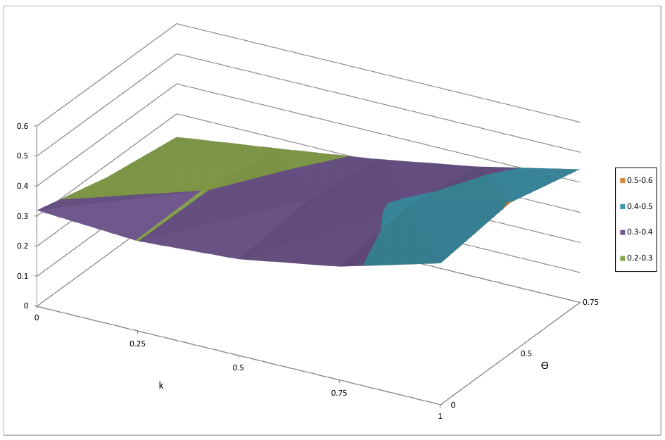
The color scale tops in a band of 0.5 to 0.6, and that band is a small patch at k near 1, on the boundary of the search. The text names the cell k equal to 1 and O equal to 0.5. The notes under the in-sample table and the out-of-sample table both name O equal to 0.6. The surface was maximized inside the fit window, and the paper then names two smoothing weights for the same test. The best cell sits on the k equal to 1 boundary. She describes k above 1 as the more aggressive book, and that region sits outside the search.
WTI is a NYMEX future and Brent is an ICE future. Dubai in this basket is a Platts assessment, a published price. The daily study rolls the front-month pair on the first day of the trading month. The weekly study is silent on the roll. The 0.25 percent charge is the same at a 100 dollar barrel and at a 40 dollar barrel, because c multiplies a position built by treating a dollar gap as a pure number.
I am against shipping the printed cell. Re-estimate the cointegrating vector on a window that ends before the week you trade, so the break test's sample closes before the year you report. If the best k sits on the edge of the grid, extend the grid until you are on a plateau. Drop the leg whose t-statistic is -0.50, and drop the leg that is an assessment. The variance ratio can stay on the desk as a description of the residual she built: at thirty weeks it is about one fifth of the random-walk benchmark. The hedge ratio that produced the residual is a 2005 to 2007 estimate, and Table 3 is where it stops.
KEY POINTS
- Build the mispricing as WTI minus a cointegration fit on Brent and Dubai. The weekly R-squared is 0.995.
- Score the book by the derivative of the terminal variance. On a 20-week OU with alpha 0.2, that derivative is about 400 times steeper with five weeks left than at the start.
- Fade last week's residual with minus its sign times the absolute residual to the power k. A 4 dollar gap at k equal to 1 is a position of -4.
- Re-fit when the Quandt statistic rejects stable weights. The weekly statistic is 61.27, dated 14 February 2005, and Dubai's weight changes sign.
- Treat the out-of-sample 30.26 percent in 2009 as one year that has to stand on its own.
References
- Why Systems Work Until They Don't
- Stocks and Bonds Predict FX — But Only in Emerging Markets
- Stat-Arb Is a Clustering Problem: Multi-View Spectral > Any Signal
- Mean-Reverting Statistical Arbitrage Strategies in Crude Oil Markets, Viviana Fanelli
A note on AI. The ideas, research, analysis, and conclusions in this article are my own. I use AI tools to help with editing and wordsmithing, because English is not my first language, and I am not shy about that. AI-generated ideas and AI-assisted writing are not the same thing: the first is empty slop from a generic prompt, the second is a tool for communicating years of real research more clearly. Judge the work by its substance, not by whether software helped polish the prose.