9.12 Why Your Arbitrage Solver Crashes at 99 Cents: Barrier Frank-Wolfe
The clean arbitrage solver crashes near 99 cents because the log gradient blows up at the boundary. The barrier fix shrinks the shape off 0 and 1, converging slower but actually finishing.
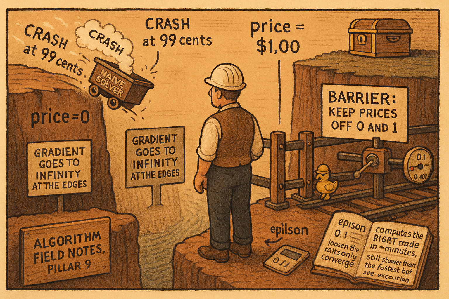
The projection converges in theory. The article "Frank-Wolfe: Solving a Quintillion-Vertex Problem in 100 Steps" ended on a caveat that sounds academic and is not: the convergence guarantee needs a finite Lipschitz constant, and on the log-scoring market maker Polymarket runs, that constant is infinite. Point the clean algorithm at a real market and it works fine until a price drifts toward 99 cents or 1 cent, then it overflows or oscillates and never returns a trade. Prediction markets live at those extremes, near-certain events and near-impossible ones, which is exactly where the naive solver dies. The fix is small in concept and mandatory in practice.
The gradient explodes at the boundary
The market maker's cost function, for a log-scoring rule, has a conjugate equal to negative entropy. Its gradient and its curvature are what the solver leans on, and both misbehave as any price approaches zero.
$$ \nabla C^*(p) = \big(\ln \mu_1 + 1,\; \ldots,\; \ln \mu_n + 1\big), \qquad \nabla^2 C^*(p) = \text{diag}\!\left(\tfrac{1}{\mu_1},\; \ldots,\; \tfrac{1}{\mu_n}\right) $$
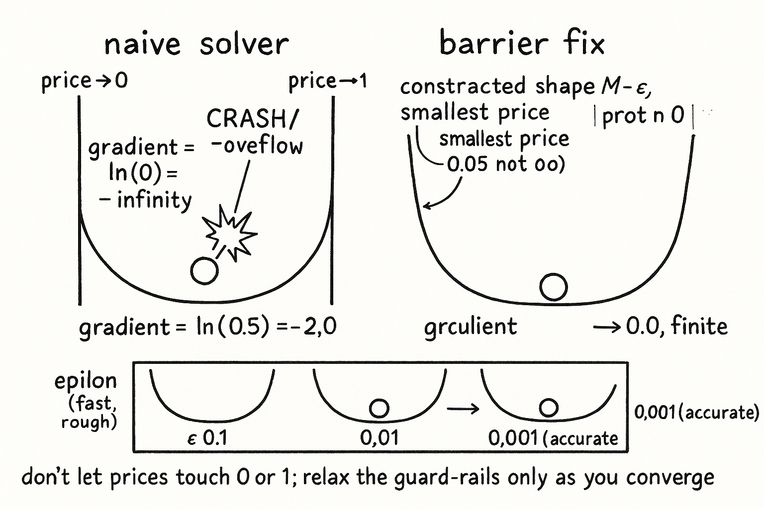
The gradient carries a natural log of each price. As a price mu approaches zero, the log runs to negative infinity. The curvature carries one over each price, which runs to positive infinity. And the arbitrage-free shape has corners where some coordinates are exactly zero, because those are outcomes where a security does not pay. March the iterates toward such a corner and the gradient and curvature both blow up. The Lipschitz constant, the ceiling on how fast the gradient can change, is the largest curvature anywhere in the shape, and near those corners it is unbounded.
$$ L = \sup_{p \in M} \|\nabla^2 C^*(p)\| = +\infty $$
Once L is infinite, the convergence bound from the previous article is void. It divided by nothing useful. There is no promise the iterates settle, and in practice they do not: a price near zero behaves like dividing by zero, and the solver either throws a floating-point overflow or bounces between wild step sizes without homing in. This is not a rare pathology. It fires every time a security resolves toward 0 or 1, which on a prediction market is a daily event, not a corner case.
Do not let prices touch the wall
The fix reads like risk management, because it is. Do not let prices get arbitrarily close to 0 or 1. Shrink the feasible shape slightly inward, toward a point known to sit safely in the interior, so the smallest price the solver can reach is bounded away from zero.
$$ M_\varepsilon = (1 - \varepsilon)\, M + \varepsilon\, u, \qquad u \in \text{int}(M) $$
The contracted shape M-epsilon is the original shape pulled a fraction epsilon of the way toward an interior point u. Every point in it is a blend, mostly the original shape, a sliver of the safe interior point. That sliver is enough to keep every coordinate off zero.
The numbers make it concrete. Binary market, corners at (1,0) and (0,1), interior point u at (0.5, 0.5), contraction epsilon of 0.1. The corner (1,0) gets pulled to 0.9 times (1,0) plus 0.1 times (0.5,0.5), which is (0.95, 0.05). The corner (0,1) moves to (0.05, 0.95). The contracted shape is the segment between those, and its smallest coordinate is 0.05, never zero. The gradient there is the log of 0.05 plus 1, about 2.0 in magnitude, a normal finite number instead of negative infinity. The curvature ceiling becomes finite too.
$$ L_\varepsilon \le \frac{1}{\varepsilon \cdot \min_j u_j} = O(1/\varepsilon) $$
The bound on curvature is now one over epsilon times the smallest interior coordinate. Finite for any positive epsilon, so the convergence guarantee from the previous article applies again on the contracted shape. The interior point u is not something you invent; the initialization routine from the article "Frank-Wolfe: Solving a Quintillion-Vertex Problem in 100 Steps" already produced it as the average of the starting corners, with every unsettled coordinate strictly between 0 and 1. This is why that routine bothered to compute an interior point instead of just a starting vertex.
The tradeoff, and the schedule that resolves it
Contraction is not free. Shrink too hard and you converge fast to the wrong answer; shrink too little and you converge slowly to the right one.
A large epsilon, say 0.1, gives a small curvature ceiling and fast convergence, but the contracted shape is a poor stand-in for the real one, so the trade you compute is off. A small epsilon, say 0.001, keeps the contracted shape almost identical to the real one, so the target is accurate, but the curvature ceiling is large and progress crawls. Pick one fixed epsilon and you are stuck choosing between fast-and-wrong or slow-and-right.
The resolution is to move epsilon over time: start large for speed, shrink toward zero as the algorithm homes in, so early iterations move fast on a rough target and late iterations refine on an accurate one.
$$ \varepsilon_t = \min\!\left\{ \frac{g(p_t)}{-4\,g_u},\; \frac{\varepsilon_{t-1}}{2} \right\} \text{ if that ratio } < \varepsilon_{t-1}, \text{ else hold } \varepsilon_{t-1} $$
The rule ties the shrink to progress. The g is the Frank-Wolfe gap from the previous article, the profit-still-on-the-table number. The g-u is the same gap measured toward the interior point, always negative. Their ratio measures how well the algorithm is converging relative to that interior direction. When the ratio is small, meaning good progress, epsilon halves. When progress stalls, epsilon holds. The schedule is automatic; nobody hand-tunes it per market.
| Phase | Iterations | Epsilon | What happens |
|---|---|---|---|
| Early | 1 to 10 | around 0.1 | fast progress toward a rough trade |
| Middle | 10 to 50 | 0.01 to 0.05 | refinement |
| Late | 50 to 150 | around 0.001 | high-precision convergence |
As epsilon goes to zero the contracted shape converges to the real one and the iterates converge to the true projection. The overall rate is 1 over the square root of t, slower than the 1 over t of the standard method. Slower and it converges beats faster and it crashes. The standard method on this class of problem does not converge at all.
The full pipeline, and the honest cost
Assemble the three computational articles and the structural arbitrage engine is complete. Initialization runs in under a second and hands over the starting corners and the interior point. Barrier Frank-Wolfe then runs 50 to 150 iterations; each iteration is a millisecond convex subproblem, a 1-to-30-second integer-program oracle call, and a negligible epsilon update and stop check. Total wall-clock, minutes to about half an hour. Then the profit check: if the guaranteed profit, the divergence minus the gap, clears 5 cents, execute the trade the projection produced; otherwise there is no arbitrage worth the execution risk.
Read the timing again and the strategic picture sharpens. Minutes to thirty minutes to compute a trade, on a platform where prices move within a single Polygon block, roughly two seconds. The barrier fix is what makes the answer correct. It does nothing to make it fast enough to beat the fastest bots, and it does nothing about whether both legs fill once you commit. The 5-cent floor exists because the theoretical profit that clears it still has to survive the slippage, fees, and partial-fill risk cataloged in the article "Execution Is Part of Expected Value," and a large fraction of trades that pass the math fail there. Barrier Frank-Wolfe closes the numerical gap in the theory. The gap between a correct trade and a captured one stays wide open, and it is where most of this pillar's later warnings live.
KEY POINTS
- On a log-scoring market maker the gradient carries a natural log of price and the curvature carries one over price, so both blow up as a price nears zero. The arbitrage-free shape has corners at exactly zero, so naive Frank-Wolfe hits an infinite Lipschitz constant and its convergence guarantee is void.
- The failure is not rare: a price near zero behaves like dividing by zero, causing overflow or oscillation, and it fires every time a security resolves toward 0 or 1, which is constant on prediction markets.
- The fix contracts the shape a fraction epsilon toward a safe interior point, so the smallest reachable price is bounded away from zero. With epsilon 0.1 a binary market's corners move to (0.95, 0.05), the gradient becomes about 2.0 instead of negative infinity, and the curvature ceiling becomes finite.
- The interior point comes free from the initialization routine, which is why that routine computed an interior point rather than just a starting vertex.
- A fixed epsilon forces a choice between fast-and-wrong and slow-and-right, so epsilon shrinks on a schedule tied to convergence progress: around 0.1 early, 0.001 late. The rate is 1 over root t, slower than standard Frank-Wolfe but it converges, which the standard method does not.
- The full pipeline (init under a second, 50 to 150 barrier iterations, minutes to 30 minutes, then a 5-cent profit floor) produces a correct trade. It does not make the trade fast enough to beat the quickest bots or guarantee both legs fill; those leaks live in the execution articles.