5.66 Stochastic Control for Market Making: The Practitioner Deck

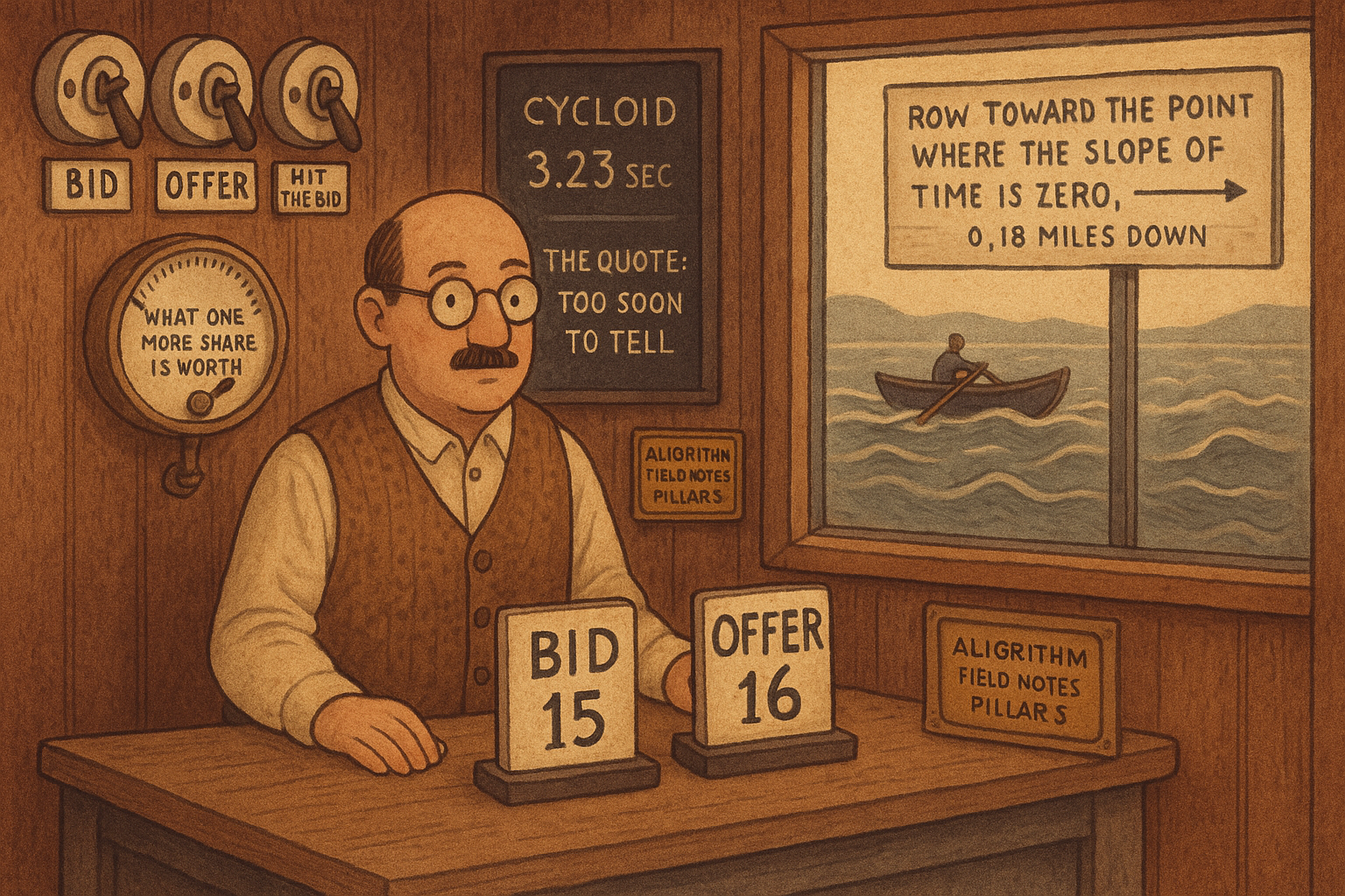
Doug Borden, in Knight Capital's electronic trading group, wrote a maker's quote as two prices and two weights for a Columbia workshop on 19 November 2010. You show 100 shares on the bid and 100 shares on the offer. Each price starts at the mid, adds a fitted weight times a short-dated forecast, subtracts a fitted weight times that name's marginal contribution to the book's risk, and then steps away from the mid by the average half-spread. He puts the payment for doing this at 0.01% to 0.10% per position, about the width of the bid-offer, and you earn it by buying while the market falls. The weights are a stable backtest, and his own weakness list says the edge cases come out badly. His policy is four orders, each live or dead, chosen from the inventory and the book as they stand right now.

Two weights shift the center, and the size stays 100

The forecast weight and the risk weight are the whole parametric quote. Marginal contribution to risk, call it MCR, is the signed amount this name adds to the book's risk, in dollars of price. Positive MCR means the position is adding long risk, so subtracting it cheapens both the bid and the offer. That sign is required by the formula as he wrote it. An unsigned risk number would cheapen the quote when you are short, which is the wrong way.

$$ P_{\text{buy}} = M + A F - B \,\mathrm{MCR} - h, \qquad P_{\text{sell}} = M + A F - B \,\mathrm{MCR} + h $$

M is the mid in dollars. F is your dollar forecast of the mid. A is the fraction of that forecast you let into the quote, fit on a backtest. B is the fraction of MCR you let in, fit the same way. h is the average half-spread in dollars. The center of the quote is M + A F - B MCR. The half-spread opens a bid below that center and an offer above it. Size does not enter. He fixes it at 100 shares each side.

Worked on a 40 dollar mid, so a one-cent half-spread is 0.025% of price and the two-cent full spread is 0.05%, inside the band he quoted. He keeps the spread at a constant width and names Citigroup as a stock that traded that way. The worked prices use a 40 dollar mid so the penny spread lands inside his return band. Take A = 0.5 and B = 0.5, both arbitrary stand-ins for weights the deck says you backtest and does not print. Forecast F = 0.04 dollars. With MCR = 0.04 the two shifts cancel: the center is 40.00 + 0.02 - 0.02 = 40.00, the bid is 39.99, and the offer is 40.01.

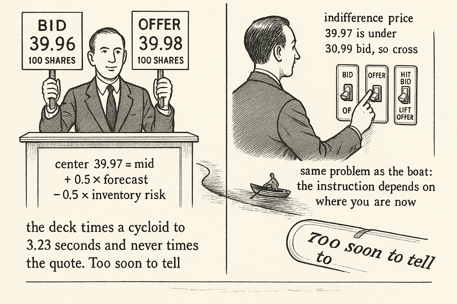
Now you are longer and MCR rises to 0.10. B times MCR is 0.05. The center falls to 40.00 + 0.02 - 0.05 = 39.97. The bid is 39.96 and the offer is 39.98. Both prices dropped 3 cents, the spread is still 2 cents, and the size is still 100 by 100. That parallel shift is the skew. The old article "The Three Pillars of Market Making: Fair Price, Spread, Skew" stacks the same three pieces in the same order: a center, a lean, then a width. Borden folds the lean into the center and leaves the width for last. That old article ranks the lean last and the center first. He takes the forecast as known and puts the mathematics on the inventory charge.

He lists two strengths, that the rules are intuitive and the fit tends to be stable, and three weaknesses: edge cases come out badly, the rule set grows until you cannot see it, and the rules do not adapt when the market's structure changes. The edge case that matters is the one the two prices cannot express. Nothing in the formula ever tells you to pull the bid and hit it.

The fastest landing is where the slope of time is zero

He builds the step from a point, to a curve, to a policy, on one river. Jack is half a mile from the far bank. Jill is 2 miles downstream. He rows at 3 miles an hour and, once across, runs at 9. The decision is a single number: how far downstream to aim the boat.

$$ T(x) = \frac{\sqrt{\tfrac{1}{4} + x^{2}}}{3} + \frac{2 - x}{9}, \qquad \frac{dT}{dx} = \frac{x}{3\sqrt{\tfrac{1}{4} + x^{2}}} - \frac{1}{9} $$

T is hours. x is miles downstream along the far bank. The first term is the diagonal row, half a mile across and x miles down, at 3 miles an hour. The second term is the run that remains, at 9 miles an hour. Set the derivative to zero and the fraction of the diagonal that points downstream equals 1/3, which is the rowing speed divided by the running speed:

$$ \frac{x}{\sqrt{\tfrac{1}{4} + x^{2}}} = \frac{1}{3} $$

Square both sides. Nine x squared equals 1/4 plus x squared, so eight x squared equals 1/4, and x squared equals 1/32. The root is the square root of 1/32, which is 0.1768 miles to four decimals. The slide prints 0.1767 miles. At 0.1767 the derivative is about -0.000043 hours per mile, not exactly zero. The printed root is the exact root with a digit cut off. The time at either figure is 22.76 minutes, so the cut does not move the answer you would use.

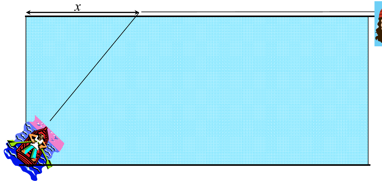
Rowing straight across, x = 0, takes 0.5/3 hours on the water plus 2/9 hours on the bank, which is 0.1667 + 0.2222 = 0.3889 hours, or 23.33 minutes. At the root the diagonal is the square root of 0.28125, or 0.5303 miles. Rowing it takes 0.1768 hours. The run is 1.8232 miles and takes 0.2026 hours. The sum is 0.3794 hours, 22.76 minutes, about 34 seconds faster than straight across. Aiming the boat at the point beside Jill, x = 2, takes the square root of 4.25 divided by 3, which is 0.6872 hours, or 41.23 minutes. The optimum is a small downstream aim because the run is three times the row.

A route is a curve, and the curve has to satisfy Euler-Lagrange

Give the river a current that depends on where you are across it, and close the bank to running. The decision stops being a landing point. It becomes a function y(x), the path across. The time of a path is an integral of a Lagrangian L, and the path that extremizes the time satisfies the Euler-Lagrange equation. L here is the time incurred per mile downstream, a function of the path and of its slope.

$$ \frac{d}{dx}\frac{\partial L}{\partial y'} - \frac{\partial L}{\partial y} = 0 $$

The first term is how the slope's contribution to time changes as you move downstream. The second subtracts how time changes when the path itself sits higher or lower in the current. A path is optimal when those two stay in balance at every point downstream. For the landing-point problem there is no slope inside an integral. L is T, and the same statement collapses to dT/dx = 0. That is the 0.1768 mile root again. The freshman condition is the sophomore condition with the path squeezed down to a point.

The slide also prints an integrand for the current. Transcribe it as he printed it.

$$ T = \int_{0}^{2} \sqrt{ \frac{(1+y'^{2})^{3/2}}{(9+v(y)^{2})\sqrt{1+y'^{2}} - 6v(y)} } \, dx $$

v(y) is the current in miles per hour. The 9 is the square of the 3 mile-an-hour row, a speed squared. The 6v(y) term is twice the rowing speed times the current, a speed. The denominator subtracts a speed from a speed squared. Those units do not close. The slide may have a typesetting error in the integrand. Solve the Euler-Lagrange equation, and leave this integral out of the code.

Shares change only when a switch is on

The same ladder, one step further, is the quote. The river with rapids no longer has a path you can choose in advance. Jack needs a rule that reads where the boat is now and says which way to row. For the book, where the boat is now is the mid, the two fill rates, and the inventory. The rule says which of four orders to have live.

The mid follows what he calls algebraic Brownian motion. The equation is arithmetic. The mid moves by a dollar drift plus a dollar shock, not by a percent. mu(t) is that drift, and he takes it as known. That is your forecast, brought in from outside. sigma is the dollar volatility per square root of time.

Limit fills are not constant. A sell-fill rate and a buy-fill rate each tug back toward a baseline rate v-naught, and a single shock knocks them in opposite directions. beta is the tug, per unit time. zeta is the size of the shock to the fill rate. The deck writes a variant sigma in the fill equations and zeta in the partial differential equation. They are the same object.

$$ dS = \mu(t)\,dt + \sigma\,dz, \qquad dv_s = \beta(v_o - v_s)\,dt + \zeta\,dz, \qquad dv_b = \beta(v_o - v_b)\,dt - \zeta\,dz $$

Worked on the sell-fill tug alone. Let beta = 0.2 per second, v-naught = 1 share per second, and v-sell = 4 after a burst. The drift is 0.2 times (1 - 4) = -0.6 shares per second, per second. One second later the expected sell-fill rate is 3.4 if no new shock arrives. The burst fades. A parametric shade you leave on all afternoon will outlive the thing that caused it.

The opposite signs on the one shock are the adverse selection he named at the start. A shock that lifts the mid speeds the offer fills and slows the bid fills. You sell into the rise. There is no market impact: your orders do not move the mid and do not move these rates.

What you control is participation. lambda-b is 1 when a buy limit sits on the bid and 0 when it does not. lambda-s is the same switch for a sell limit on the offer. m-b and m-s are the switches for a market buy and a market sell. A limit earns the half-spread. A market order pays it. Market orders fill at a constant rate f-naught, and he only says that rate exceeds v-naught. He does not print either number.

Inventory N, in shares, moves with whichever switches are on.

$$ dN = \big[-\lambda_s v_s + \lambda_b v_b - m_s f_o + m_b f_o\big]\,dt $$

Selling cuts the position. Buying adds to it. With both limits on, both market switches off, and each limit filling 1 share per second, the change in N is -1 + 1 = 0. Cash per second is the ask times the sell rate minus the bid times the buy rate. On the 40 dollar mid with a one-cent half-spread that is 40.01 minus 39.99, so 0.02 dollars per second. You are flat, and you are earning two cents a second.

After the burst, take v-sell = 4 and v-buy = 0, limits still on, markets still off. Inventory changes at -4 shares per second. Cash in is 40.01 times 4 = 160.04 dollars per second. Mark the four shares at the mid and they are worth 160.00. The spread capture is 0.04 dollars per second. You moved 160 dollars of stock to earn 4 cents, and the same shock that filled the offer is the one that marked the mid up. That 4 cents is the payment for having sold into it.

The second-order terms in his equation for the value function do not match this shock. With one Brownian motion and a buy-fill loading of minus zeta, Ito's formula puts a minus on the mid-versus-buy-fill cross term and a minus on the buy-fill-versus-sell-fill cross term. The slide prints both with a plus.

$$ \text{slide: } +\sigma\zeta \frac{\partial^{2}H}{\partial S\,\partial v_b} + \zeta^{2}\frac{\partial^{2}H}{\partial v_b\,\partial v_s} \qquad \text{Ito: } -\sigma\zeta \frac{\partial^{2}H}{\partial S\,\partial v_b} - \zeta^{2}\frac{\partial^{2}H}{\partial v_s\,\partial v_b} $$

H is the value of the maximized objective from the current state forward. Take sigma = 0.005 dollars per square-root second and zeta = 1 share per second per square-root second, the second figure arbitrary and used only for this check. Their product is 0.005. If the mixed derivative of H with respect to the mid and the buy-fill rate equals 1, the slide adds +0.005 to the generator and the minus in the buy-fill shock adds -0.005. Keep his signs if you are transcribing the slide. Do not flip them quietly and call it the same equation. The participation rules below do not use these terms. The controls sit in the drift of inventory and in the cash, not in the diffusion.

The objective charges variance for as long as you hold

The quantity he maximizes is risk-adjusted cash over a horizon from 0 to T. eta is the risk aversion, in per dollar, so that a variance charge in dollars squared per unit time becomes dollars per unit time and can sit next to the cash.

$$ U = \int_{0}^{T} \Big[ (S+\delta)\lambda_s v_s - (S-\delta)\lambda_b v_b + (S-\delta)m_s f_o - (S+\delta)m_b f_o - \eta\sigma^{2} N^{2} \Big]\,dt $$

delta is half the constant spread, so the ask is S + delta and the bid is S - delta. A live sell limit earns the ask times the sell-fill rate. A live buy limit pays the bid times the buy-fill rate. A market sell earns the bid times the faster market-order rate. A market buy pays the ask times that rate. The last term is the rent on the position: variance of the inventory's dollar move per unit time, times eta.

He does not print eta. Use 0.001 per dollar, and use sigma = 0.005. A 30% annual move on a 40 dollar stock is about 12 dollars a year, and a trading year of 252 sessions of 6.5 hours has square root about 2,428 seconds, so the dollar volatility per square-root second is about 0.0049. The 0.005 is that scale, rounded. The two-sided capture above was 0.02 dollars per second. Set the penalty equal to that capture and solve for N.

$$ \eta \sigma^{2} N^{2} = 0.02 $$

eta times sigma squared is 0.001 times 0.000025 = 2.5 times 10 to the minus 8. N squared equals 0.02 divided by that, which is 800,000. N is the square root of 800,000, or 894.4 shares. At 894 shares the charge is 0.01998 dollars per second, against the 0.02 capture. Past that size the running penalty eats a one-share-each-side market even before the adverse shock shows up. At 500 shares the same charge is 0.00625 dollars per second, about a third of that capture.

The general boundary condition says H at the horizon equals a terminal payoff B. The stock slides never set B. A position you still hold at T has been charged for variance along the way, and the written objective assigns the leftover a value of zero. If you want a cost for crossing out at the close, you have to put that term in yourself.

Each order turns on when the indifference price clears the touch

The spread is frozen. The prices on offer are the bid at S minus delta and the ask at S plus delta. You choose whether to stand on each, and whether to cross. Because each switch enters the objective linearly, the optimum is at 0 or at 1. He calls the resulting rule a generalized Heaviside step in the state and in the gradient of H. Operationally it is four comparisons. The indifference price is the derivative of H with respect to N: what one more share is worth, in dollars, inside the maximized objective.

$$ \begin{aligned} \lambda_s &= 1 \text{ when } \partial H/\partial N < S+\delta, \\ \lambda_b &= 1 \text{ when } \partial H/\partial N > S-\delta, \\ m_s &= 1 \text{ when } \partial H/\partial N < S-\delta, \\ m_b &= 1 \text{ when } \partial H/\partial N > S+\delta. \end{aligned} $$

You offer passively when a share is worth less to you than the ask you would receive. You bid passively when a share is worth more than the bid you would pay. You hit the bid only when a share is worth less than that bid, and you lift the offer only when a share is worth more than that ask. A positive fill rate scales the dollars per second and leaves the sign with the indifference price. Inventory enters only by moving the indifference price. The penalty has no separate switch.

The deck leaves H unsolved. The numbers below put the parametric center in the slot where the derivative of H with respect to N would sit, as a reading of the inequalities.

On the 40 dollar name, delta = 0.01, so the bid is 39.99 and the ask is 40.01. Let the limit rates be 1 share per second and let f-naught be 5, arbitrary except that 5 exceeds 1, which is all he required. At an indifference price of 40.00 the sell-limit coefficient is 1 times (40.01 - 40.00) = 0.01 dollars per second, and the buy-limit coefficient is 1 times (40.00 - 39.99) = 0.01. Both limits are on. The market-sell coefficient is 5 times (39.99 - 40.00) = -0.05, and the market-buy coefficient is 5 times (40.00 - 40.01) = -0.05. Both crosses are off. The quote earns the half-spread.

At an indifference price of 39.97, the long center from the two-weight quote, the coefficients are 0.04 for the sell limit, -0.02 for the buy limit, 0.10 for the market sell, and -0.20 for the market buy. The offer stays up. The bid comes off. You also sell at 39.99, because 39.99 exceeds 39.97 by 2 cents, and at 5 shares a second that gap is 0.10 dollars per second of objective. The buy limit would cost you 0.02 dollars per second, so it stays off.

Look at the market-sell panel. The step is on to the left of the dashed line at 39.99, and the dotted line at 39.97 sits in that region.

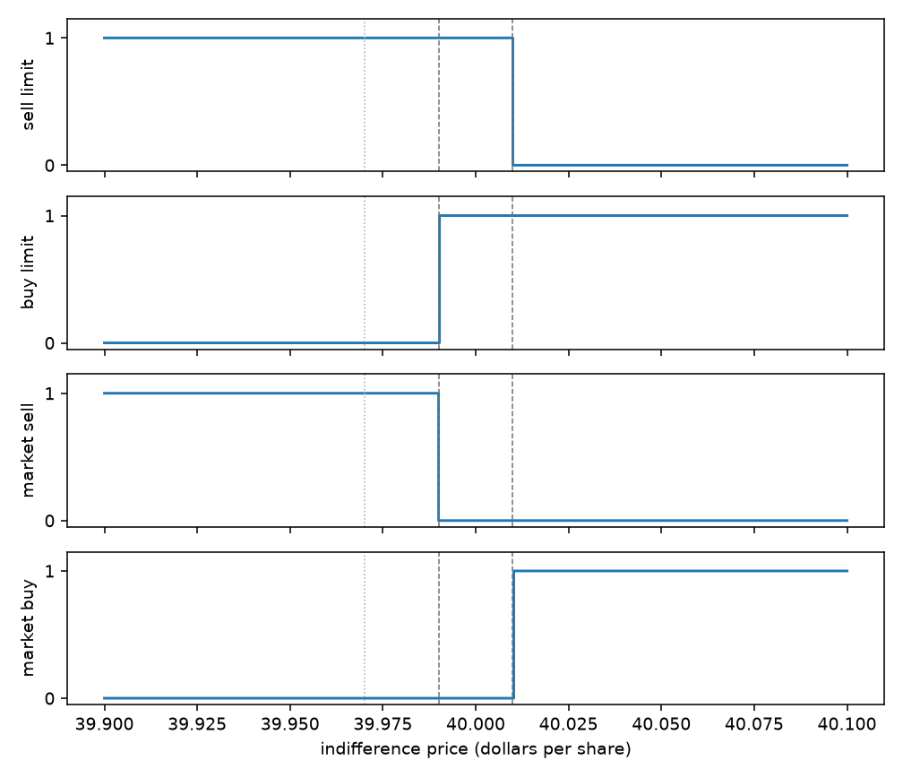
The two-weight quote, handed the same 39.97 center, is still bidding 39.96 and offering 39.98, 100 shares a side. A bid at 39.96 would be a buy below an indifference price of 39.97, which is a sensible order inside a menu that lets you pick any price. That menu has no market sell. The control menu has the market sell and cannot post 39.96, because the spread is glued at two cents. Same inventory number, two different sets of legal orders. His hope is that the switches handle the edge case the weights miss. The deck does not run them against each other.

A market sell and a buy limit need opposite sides of the bid, so they are never on together. A market sell and a sell limit are on together whenever the indifference price is below the bid. Receiving the ask on the offer is a better sale than hitting the bid, so that offer stays up too.

He times the slide, and he leaves the book untimed

Look at the red curve, the cycloid.

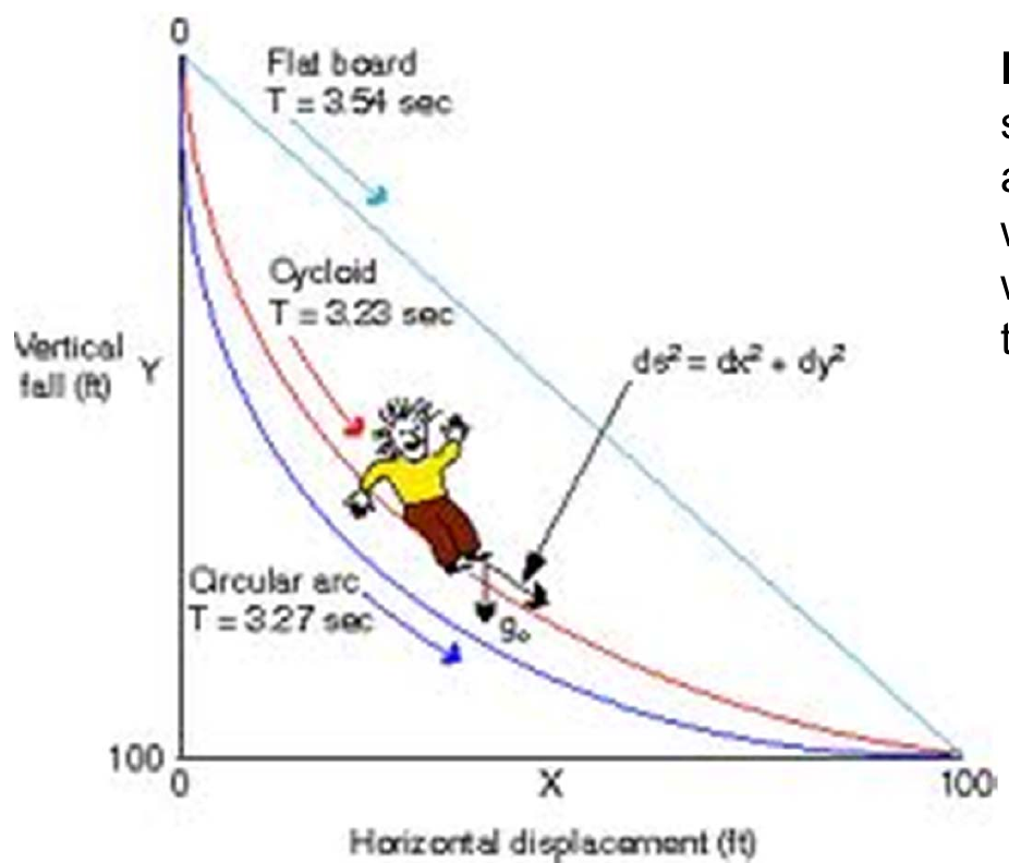
The flat board takes 3.54 seconds, the circular arc 3.27, and the cycloid 3.23. The cycloid beats the arc by 0.04 seconds and the board by 0.31 seconds. The board's time recomputes. The run is 100 times the square root of 2, or 141.42 feet, at 45 degrees. With gravity at 32 feet per second squared the acceleration along the board is 22.63 feet per second squared, and the time is the square root of 12.5, which is 3.535 seconds and rounds to the printed 3.54. The arc and the cycloid stay the figure's labels.

The quoting question gets one sentence from him. The partial differential equation is solvable with the tools physics and derivatives desks already had in 2010, a solver on the order of a second is about a thousand times too slow for the decision, and whether the policy makes money is, in his words, too soon to tell.

Four comparisons are what you can run in time

Knight's 2009 tape averaged 600,000 trades an hour, about 167 a second across the firm. Run the four comparisons on that path, fed by an indifference price you computed on a grid beforehand, or by a price you are willing to stand behind. A solver on the order of a second is about a thousand times too slow for a tape at that rate. Precomputing on a second box still leaves the live step as those four inequalities.

I am against reading the untimed policy as a pending improvement on the two weights. The weights pick prices at a size glued to 100 shares. The switches pick participation at a frozen spread, and the size that comes back is whatever the fill rate delivers while the switch is on. Neither menu chooses size. If you want size, you still write it yourself.

The forecast has to come from you. mu(t) enters as a known function. A wrong center moves every threshold, because each comparison is the indifference price against a bid or an ask built from the mid. Spend the work on that center before you spend it on the step. The old article "The Three Pillars of Market Making: Fair Price, Spread, Skew" already ranks the pieces that way.

A backtest of this equation misses the fill you never got. The fill rates do not depend on anyone else's inventory, so a market order that misses you leaves the state unchanged. The old article "Market Making With Competitors You Can't See" puts that missed fill onto the other maker's inventory, and their next quote moves because of it. The rates themselves are a process you assumed. The old article "Why Market-Making Simulations Don't Work" is why a smooth fill intensity cannot stand in for a limit that was never on the book. Borden's modeling choice is one line, no market impact, and the performance line is blank. The equation is a prior on when to cross. Production markouts are the test. The fill-rate shock is also free to print a negative rate, since nothing clips the mean-reverting pair at zero. Clamp it. A negative rate reverses the sign of the switch.

KEY POINTS

• Write both prices off one center, mid plus A times the forecast minus B times signed marginal risk, then open by the half-spread. With A and B at 0.5, a 0.04 dollar forecast and a 0.10 long-risk contribution put the bid at 39.96 and the offer at 39.98, still 100 shares by 100.
• Check a point optimum before you trust a path. The river's derivative is zero at 0.1768 miles, the square root of 1/32. The slide's 0.1767 is that root with a digit cut off, and either one takes 22.76 minutes against 23.33 straight across.
• Switch orders by comparing the indifference price to the touch. At 39.97, against a 39.99 bid, a market sell filling 5 shares a second adds 0.10 dollars per second, and the buy limit subtracts 0.02.
• Charge the position at eta times sigma squared times N squared. At eta of 0.001 per dollar and sigma of 0.005, the charge matches a 0.02 dollar-per-second two-sided capture when you hold 894 shares.
• Treat the quoting policy as untimed. His only clock is the slide, 3.23 seconds against 3.27 and 3.54, and his line on the book is that a solver on the order of a second is about a thousand times too slow, and that it is too soon to tell.

References

• The Three Pillars of Market Making: Fair Price, Spread, Skew
• Market Making With Competitors You Can't See
• Why Market-Making Simulations Don't Work
• Stochastic Control Theory & Automated Market Making, Doug Borden

A note on AI. The ideas, research, analysis, and conclusions in this article are my own. I use AI tools to help with editing and wordsmithing, because English is not my first language, and I am not shy about that. AI-generated ideas and AI-assisted writing are not the same thing: the first is empty slop from a generic prompt, the second is a tool for communicating years of real research more clearly. Judge the work by its substance, not by whether software helped polish the prose.