9.1 Convex Geometry for Traders: Polytopes, Hyperplanes, Projection, and Why KL Beats Euclidean

Most traders reach for a forecast the moment they open a prediction market. They read the news, form a view, and buy the side they like. That instinct is the one this whole pillar argues against, and the argument is geometric before it is financial. The cleanest money on Polymarket and Kalshi comes from prices that contradict each other, not from prices that turn out wrong. To see those contradictions you need a small vocabulary of convex geometry: convex sets, hulls, polytopes, hyperplanes, gradients, conjugates, and two ways of measuring distance. Learn the vocabulary here, on toy examples, and the heavy machinery of the later articles stops looking like a wall.

This is a gateway article. It teaches the words. Nothing here makes you money on its own, but every profitable idea in the pillar is written in this language, and traders who skip it end up trusting a solver they cannot read.

A price vector is a point in space

Fix a set of contracts. A US-election market might have "Candidate A wins" and "Candidate A loses" as two YES contracts, each paying $1 if its event resolves true. The prices, say $0.40 and $0.40, form a pair of numbers. Write that pair as a single point in a plane: the horizontal axis is the price of the first contract, the vertical axis the second. A market with three contracts is a point in three-dimensional space, and a market with a thousand contracts is a point in thousand-dimensional space you cannot draw but can still reason about.

That reframing is the whole trick. Once prices are points, "is this market internally consistent?" becomes "does this point sit inside a particular region?" The region has a name and a shape, and the shape is convex.

Convex sets: the shape with no dents

A set is convex when a straight line between any two points inside it stays inside it. A filled disk is convex. A crescent moon is not, because a chord between the two horns leaves the shape. A solid cube is convex; a cube with a bite taken out is not.

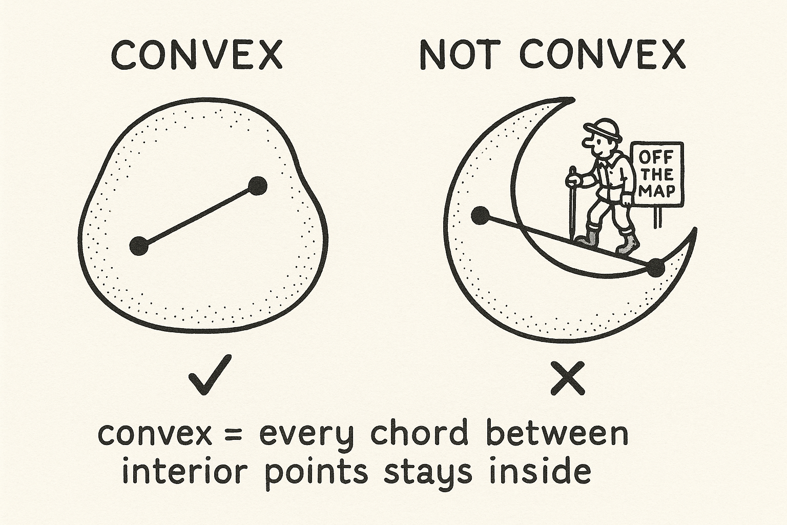
Convexity matters because the set of all sensible prices is convex, and because convex problems are the ones optimizers can solve without getting stuck in false optima. Every guarantee later in the pillar leans on it.

Convex combinations and the hull

A convex combination is a weighted average where the weights are non-negative and add to one. Two-thirds of point A plus one-third of point B lands on the segment between them, closer to A. Stretch this to many points and any weighted average with non-negative weights summing to one lands somewhere in the solid region they span.

$$ x = \lambda_1 x_1 + \lambda_2 x_2 + \cdots + \lambda_n x_n, \qquad \lambda_i \ge 0, \quad \sum_i \lambda_i = 1 $$

Read that as: pick some anchor points, assign each a non-negative weight, force the weights to sum to one, and the result is a legal blended point. The lambdas behave exactly like probabilities, because they are non-negative and sum to one. That is not a coincidence, and it is the bridge to markets: a fair price vector is a probability-weighted average of what the contracts pay in each possible outcome.

The convex hull is the smallest convex set containing a group of points. Hammer nails into a board at each point, stretch a rubber band around the outside, let it snap tight, and the shape it encloses is the hull. Every point inside is some convex combination of the corner nails.

Polytopes: hulls with flat sides and corners

A polytope is a convex hull of finitely many points. In two dimensions it is a polygon, in three a polyhedron, in higher dimensions a polytope you name but do not sketch. It has flat faces and a finite count of sharp corners called vertices.

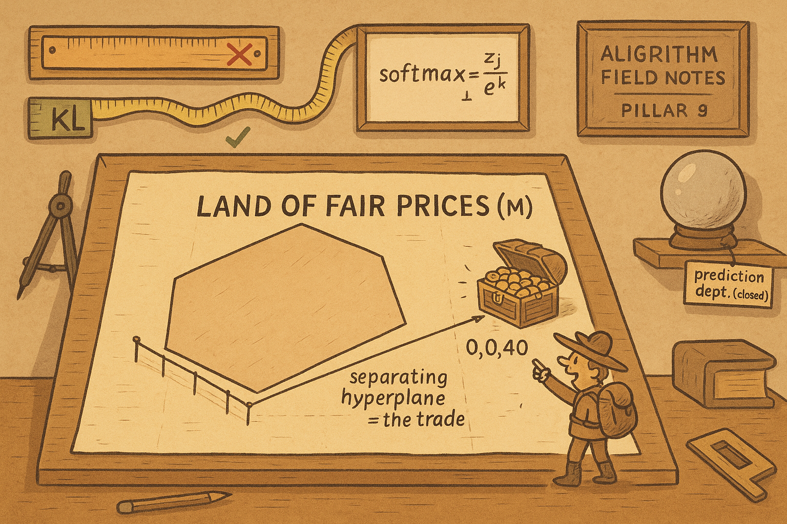
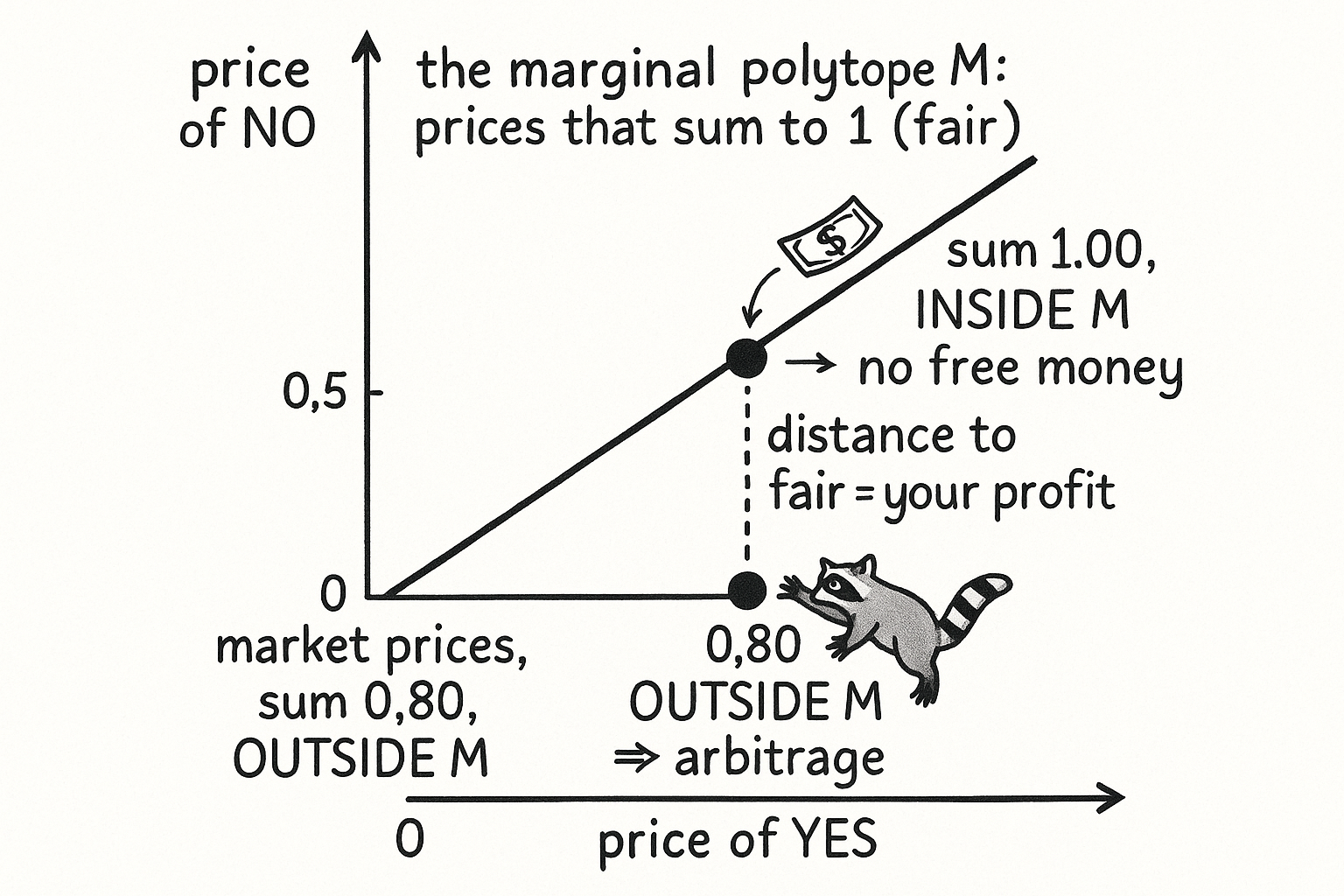
The object that runs this pillar is the marginal polytope. Its corners are the payoff vectors of the market, one corner per distinct way the world can resolve. For a single binary market the payoff vectors are (1, 0) if YES pays and (0, 1) if NO pays, so the marginal polytope is the line segment joining those two points. Every point on that segment has coordinates that sum to one.

$$ \mathcal{M} = \operatorname{conv}(\mathcal{Z}) = \Bigl\{ \sum_{\omega} \lambda_\omega \, \phi(\omega) \;:\; \lambda_\omega \ge 0,\; \sum_\omega \lambda_\omega = 1 \Bigr\} $$

Read that as: script-Z is the set of payoff vectors, one per outcome, and script-M is their convex hull. A price vector inside script-M corresponds to some honest probability distribution over outcomes. A price vector outside script-M corresponds to no probability distribution at all, which means the prices contradict themselves, which means guaranteed profit sits on the table. The entire structural half of the pillar is one membership question: is the current price point inside this polytope?

Hyperplanes: the boundary that is the trade

A hyperplane is a flat cut that splits space into two halves. In two dimensions it is a line, in three a plane, in higher dimensions a flat sheet of one dimension less than the space. Define it by a direction vector and a threshold.

$$ \mathbf{a} \cdot \mathbf{x} = c $$

Read that as: pick a direction a, and every point x whose dot product with a equals the constant c lies on the flat cut; points with a larger dot product sit on one side, points with a smaller dot product on the other. The separating hyperplane theorem says something a trader should tape to the wall: if a point sits outside a convex set, you can always slide a flat cut between the point and the set. That cut is not an abstraction. Its direction vector is the arbitrage portfolio.

Return to prices (0.40, 0.40) outside the segment. The separating direction is (1, 1): buy one YES and one NO. Cost is 0.40 plus 0.40, which is $0.80. Whatever happens, exactly one contract pays $1, so the worst-case payout is $1.00. You paid $0.80 for a guaranteed $1.00. The 20-cent gap is the separating hyperplane made cash. The direction told you what to buy; the gap told you how much you win.

Gradients and Hessians: slope and curvature

A gradient is the vector of slopes of a function, one slope per input direction. It points uphill, toward steepest increase. In a market, the gradient of the market maker's cost function gives the current prices, so "read the prices" and "read the gradient" are the same act.

A Hessian is the matrix of second derivatives. It measures how fast the slope itself changes, which is curvature. Flat curvature means prices barely move when you trade; sharp curvature means a small order swings the price hard. For the log-market-scoring-rule maker the curvature for contract i scales as one over its price.

$$ \text{Hessian entry for security } i \;=\; \frac{1}{\mu_i} $$

Read that as: when a contract trades near a price of $0.01, the curvature is about 100, and as the price crawls toward zero the curvature blows up toward infinity. That single fact is why arbitrage solvers detonate near 99-cent and 1-cent contracts, and why the later article on Barrier Frank-Wolfe exists. A price near zero behaves like a divide-by-zero waiting to happen. The Lipschitz constant, a bound on how fast the gradient can change, goes infinite exactly where real markets spend most of their time: at the edges, where events are nearly settled.

Conjugates and duality: two coordinate systems for one market

A market has two descriptions. One counts how many shares of each contract have been bought; call it the state, an unbounded vector where a trade just adds shares to a coordinate. The other reads the implied probabilities on the screen; call it the price, bounded between zero and one and summing to one. The convex conjugate, also called the Legendre-Fenchel transform, converts between them.

$$ \text{state} \to \text{price:}\quad p = \nabla C(\theta), \qquad\qquad \text{price} \to \text{state:}\quad \theta = \nabla R^*(p) $$

Read that as: apply the gradient of the cost function C to a state and you get prices; apply the gradient of its conjugate R-star to prices and you get back the state. These two moves are inverses. You need both because arbitrage math produces target prices, and an exchange only accepts orders in shares. The conjugate is the translator from "the market should be priced here" to "buy this many of these contracts."

Duality is the deeper payoff. Strong duality says certain min-max problems can be flipped without changing the answer. The trader's problem, "choose the portfolio that maximizes my worst-case profit," is a brutal combinatorial search. Flip it with duality and it becomes "find the closest fair price to the current unfair price," a geometric projection. Same answer, tractable form. That flip is the engine of the keystone result in this pillar.

Entropy, KL, and Bregman: measuring distance the right way

Distance seems obvious until it costs you money. Euclidean distance treats a move from $0.50 to $0.60 as identical to a move from $0.01 to $0.11: both are ten cents. In probability terms they are nothing alike. The log-odds, the natural scale for beliefs, barely twitches from 0.50 to 0.60 but lurches from 0.01 to 0.11.

$$ \operatorname{logit}(p) = \ln\frac{p}{1-p}, \qquad \operatorname{logit}(0.50)=0,\quad \operatorname{logit}(0.60)\approx 0.41,\quad \operatorname{logit}(0.01)\approx -4.60,\quad \operatorname{logit}(0.11)\approx -2.09 $$

Read that as: the logit turns a probability into a real number, zero at even odds and running off toward minus-infinity as the probability approaches zero. The 0.50-to-0.60 move shifts the logit by about 0.41. The 0.01-to-0.11 move shifts it by about 2.5. The second is roughly six times the information change, yet Euclidean distance calls them equal. Size a trade on that lie and you misprice the whole opportunity.

The honest ruler is entropy-based. Entropy measures uncertainty and peaks when every outcome is equally likely. Its mirror, negative entropy, is the conjugate of the log-scoring-rule cost function. The distance built from it is the Kullback-Leibler divergence.

$$ \operatorname{KL}(p \,\|\, q) = \sum_i p_i \ln\frac{p_i}{q_i} \;\ge\; 0, \qquad \text{zero only when } p = q $$

Read that as: KL sums, over every contract, the target probability times the log-ratio of target to current probability; it is always non-negative and hits zero only when the two price vectors match. KL is not symmetric and is not a true distance, but it is the distance the market maker itself uses, measured in the maker's own information units. KL is one instance of a Bregman divergence, the family of curved rulers built from any strictly convex function.

$$ D_R(p \,\|\, q) = R(p) - R(q) - \nabla R(q)\cdot(p - q) $$

Read that as: the Bregman divergence takes the value of R at p, subtracts the value at q, then subtracts the linear approximation of R at q evaluated at p; what remains is the gap between the true curve and its tangent line, a curvature-aware distance. Plug in negative entropy and it collapses to KL. Plug in one-half the squared norm and it collapses to plain Euclidean distance. Choosing the ruler is choosing the market's geometry, and for these markets the ruler is KL. Use Euclidean and your "optimal" trade is provably not optimal.

Softmax and logit: you already know the price formula

If you have trained a classifier you have used softmax, and softmax is the price function. The log-market-scoring-rule maker sets prices by exponentiating the state and normalizing.

$$ p_i(\theta) = \frac{\exp(\theta_i / b)}{\sum_j \exp(\theta_j / b)} $$

Read that as: raise e to each state coordinate divided by a liquidity parameter b, then divide by the sum so the outputs are positive and sum to one. The state vector plays the role of logits, the prices are the softmax output, and buying shares of contract i adds to that coordinate, which pushes its price up and drags the rest down. The liquidity parameter b sets how hard prices move: small b means a tiny order swings the price, large b means the book absorbs size. The price impact of buying works out to roughly the order size times p times one-minus-p over b, largest at even odds and vanishing near the extremes. A machine-learning reader arrives already fluent; the market maker is a softmax layer with a bank account.

Putting the vocabulary to work

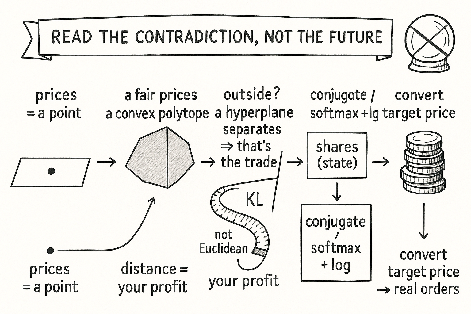
String the words together and the pillar's spine appears. Prices are a point. Fair prices form a convex polytope whose corners are payoff vectors. Ask whether the point sits inside the polytope. If it sits outside, a separating hyperplane exists, and its direction is the trade. The size of the win is the Bregman distance from the point to the polytope, measured with KL because the market maker measures in KL. Computing that distance is a projection, reachable only because duality flipped an ugly max-min into a clean minimization. Converting the target prices back into share orders uses the conjugate. Gradients read prices; Hessians warn you where the solver breaks.

Nothing in that chain requires a forecast. It requires reading contradiction in a set of numbers and acting before the market repairs itself. The pillar treats forecasting as the fifth-cleanest edge of nine and the most dangerous to size, a point the article on the nine sources of edge makes in full. Before any of that, you needed the geometry, and now you have it.

This gateway pairs with a working notebook that builds a polytope membership checker and emits the separating-hyperplane trade on the (0.40, 0.40) toy, so the words above turn into code you can run.

KEY POINTS

• Turn a market into geometry: a price vector is a single point in a space with one axis per contract, and internal consistency becomes a question of whether that point sits inside a region.
• A convex set has no dents, so a straight line between any two interior points stays inside. Convex combinations are probability-weighted averages, which is why fair prices behave like probabilities.
• The marginal polytope is the convex hull of the payoff vectors. Inside it means no arbitrage; outside it means guaranteed profit. The structural half of the pillar is one membership test.
• The separating hyperplane theorem turns geometry into a trade: if the price point sits outside the polytope, the separating direction is the portfolio to buy, and the gap it opens is the guaranteed profit.
• Gradients of the cost function are the prices; Hessians are the curvature and scale as one over price, which is why solvers explode near 1-cent and 99-cent contracts.
• The convex conjugate translates between shares (state) and prices, and duality flips the trader's worst-case-profit problem into a solvable projection onto the polytope.
• Measure distance with KL, not Euclidean. A ten-cent move near even odds and a ten-cent move near the extremes carry different information, and Euclidean distance ignores that, yielding suboptimal trades.
• Softmax is the price formula. The log-market-scoring-rule maker is a softmax layer, so a machine-learning reader already knows how prices are set.

References

• Convex Optimization - Boyd and Vandenberghe (2004)
• The Relaxation Method of Finding the Common Point of Convex Sets and Its Application to the Solution of Problems in Convex Programming - Bregman (1967)
• Arbitrage-Free Combinatorial Market Making via Integer Programming - Kroer et al. (2016)